https://learnopengl.com/#!PBR/IBL/Diffuse-irradiance

Diffuse irradiance

IBL or image based lighting is a collection of techniques to light objects, not by direct analytical lights as in the previous tutorial, but by treating the surrounding environment as one big light source. This is generally accomplished by manipulating a cubemap environment map (taken from the real world or generated from a 3D scene) such that we can directly use it in our lighting equations: treating each cubemap pixel as a light emitter. This way we can effectively capture an environment's global lighting and general feel, giving objects a better sense of belonging in their environment.

As image based lighting algorithms capture the lighting of some (global) environment its input is considered a more precise form of ambient lighting, even a crude approximation of global illumination. This makes IBL interesting for PBR as objects look significantly more physically accurate when we take the environment's lighting into account.

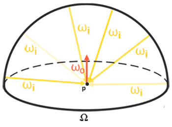
To start introducing IBL into our PBR system let's again take a quick look at the reflectance equation:

Lo(p,ωo)=∫Ω(kdcπ+ksDFG4(ωo⋅n)(ωi⋅n))Li(p,ωi)n⋅ωidωiLo(p,ωo)=∫Ω(kdcπ+ksDFG4(ωo⋅n)(ωi⋅n))Li(p,ωi)n⋅ωidωi

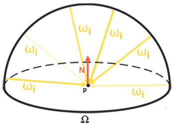
As described before, our main goal is to solve the integral of all incoming light directions wiwi over the hemisphere ΩΩ . Solving the integral in the previous tutorial was easy as we knew beforehand the exact few light directions wiwi that contributed to the integral. This time however, every incoming light direction wiwi from the surrounding environment could potentially have some radiance making it less trivial to solve the integral. This gives us two main requirements for solving the integral:

• We need some way to retrieve the scene's radiance given any direction vector wiwi.
• Solving the integral needs to be fast and real-time.

Now, the first requirement is relatively easy. We've already hinted it, but one way of representing an environment or scene's irradiance is in the form of a (processed) environment cubemap. Given such a cubemap, we can visualize every texel of the cubemap as one single emitting light source. By sampling this cubemap with any direction vector wiwi we retrieve the scene's radiance from that direction.

Getting the scene's radiance given any direction vector wiwi is then as simple as:

vec3 radiance = texture(_cubemapEnvironment, w_i).rgb;  

Still, solving the integral requires us to sample the environment map from not just one direction, but all possible directions wiwi over the hemisphere ΩΩ which is far too expensive for each fragment shader invocation. To solve the integral in a more efficient fashion we'll want to pre-process or pre-compute most of its computations. For this we'll have to delve a bit deeper into the reflectance equation:

Lo(p,ωo)=∫Ω(kdcπ+ksDFG4(ωo⋅n)(ωi⋅n))Li(p,ωi)n⋅ωidωiLo(p,ωo)=∫Ω(kdcπ+ksDFG4(ωo⋅n)(ωi⋅n))Li(p,ωi)n⋅ωidωi

Taking a good look at the reflectance equation we find that the diffuse kdkd and specular ksks term of the BRDF are independent from each other and we can split the integral in two:

Lo(p,ωo)=∫Ω(kdcπ)Li(p,ωi)n⋅ωidωi+∫Ω(ksDFG4(ωo⋅n)(ωi⋅n))Li(p,ωi)n⋅ωidωiLo(p,ωo)=∫Ω(kdcπ)Li(p,ωi)n⋅ωidωi+∫Ω(ksDFG4(ωo⋅n)(ωi⋅n))Li(p,ωi)n⋅ωidωi

By splitting the integral in two parts we can focus on both the diffuse and specular term individually; the focus of this tutorial being on the diffuse integral.

Taking a closer look at the diffuse integral we find that the diffuse lambert term is a constant term (the color cc, the refraction ratio kdkd and ππ are constant over the integral) and not dependent on any of the integral variables. Given this, we can move the constant term out of the diffuse integral:

Lo(p,ωo)=kdcπ∫ΩLi(p,ωi)n⋅ωidωiLo(p,ωo)=kdcπ∫ΩLi(p,ωi)n⋅ωidωi

This gives us an integral that only depends on wiwi (assuming pp is at the center of the environment map). With this knowledge, we can calculate or pre-compute a new cubemap that stores in each sample direction (or texel) wowo the diffuse integral's result by convolution.

Convolution is applying some computation to each entry in a data set considering all other entries in the data set; the data set being the scene's radiance or environment map. Thus for every sample direction in the cubemap, we take all other sample directions over the hemisphere ΩΩ into account.

To convolute an environment map we solve the integral for each output wowo sample direction by discretely sampling a large number of directions wiwi over the hemisphere ΩΩ and averaging their radiance. The hemisphere we build the sample directions wiwi from is oriented towards the output wowo sample direction we're convoluting.

This pre-computed cubemap, that for each sample direction wowo stores the integral result, can be thought of as the pre-computed sum of all indirect diffuse light of the scene hitting some surface aligned along direction wowo. Such a cubemap is known as an irradiance map seeing as the convoluted cubemap effectively allows us to directly sample the scene's (pre-computed) irradiance from any direction wowo.

The radiance equation also depends on a position pp, which we've assumed to be at the center of the irradiance map. This does mean all diffuse indirect light must come from a single environment map which may break the illusion of reality (especially indoors). Render engines solve this by placing reflection probes all over the scene where each reflection probes calculates its own irradiance map of its surroundings. This way, the irradiance (and radiance) at position pp is the interpolated irradiance between its closest reflection probes. For now, we assume we always sample the environment map from its center and discuss reflection probes in a later tutorial.

Below is an example of a cubemap environment map and its resulting irradiance map (courtesy of wave engine), averaging the scene's radiance for every direction wowo.

By storing the convoluted result in each cubemap texel (in the direction of wowo) the irradiance map displays somewhat like an average color or lighting display of the environment. Sampling any direction from this environment map will give us the scene's irradiance from that particular direction.

PBR and HDR

We've briefly touched upon it in the lighting tutorial: taking the high dynamic range of your scene's lighting into account in a PBR pipeline is incredibly important. As PBR bases most of its inputs on real physical properties and measurements it makes sense to closely match the incoming light values to their physical equivalents. Whether we make educative guesses on each light's radiant flux or use their direct physical equivalent, the difference between a simple light bulb or the sun is significant either way. Without working in an HDR render environment it's impossible to correctly specify each light's relative intensity.

So, PBR and HDR go hand in hand, but how does it all relate to image based lighting? We've seen in the previous tutorial that it's relatively easy to get PBR working in HDR. However, seeing as for image based lighting we base the environment's indirect light intensity on the color values of an environment cubemap we need some way to store the lighting's high dynamic range into an environment map.

The environment maps we've been using so far as cubemaps (used as skyboxes for instance) are in low dynamic range (LDR). We directly used their color values from the individual face images, ranged between 0.0 and 1.0, and processed them as is. While this may work fine for visual output, when taking them as physical input parameters it's not going to work.

The radiance HDR file format

Enter the radiance file format. The radiance file format (with the .hdr extension) stores a full cubemap with all 6 faces as floating point data allowing anyone to specify color values outside the 0.0 to 1.0 range to give lights their correct color intensities. The file format also uses a clever trick to store each floating point value not as a 32 bit value per channel, but 8 bits per channel using the color's alpha channel as an exponent (this does come with a loss of precision). This works quite well, but requires the parsing program to re-convert each color to their floating point equivalent.

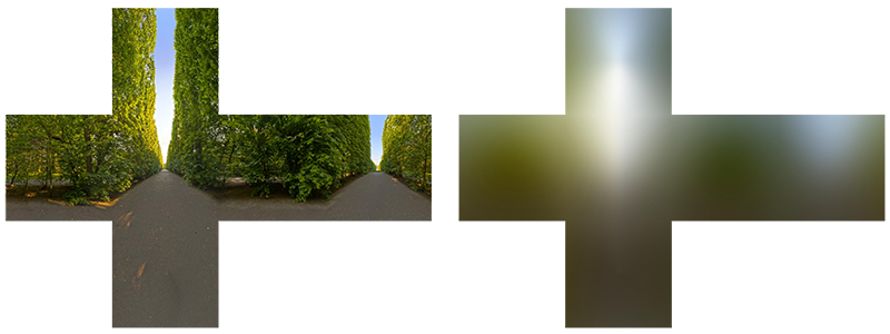
There are quite a few radiance HDR environment maps freely available from sources like sIBL archive of which you can see an example below:

This might not be exactly what you were expecting as the image appears distorted and doesn't show any of the 6 individual cubemap faces of environment maps we've seen before. This environment map is projected from a sphere onto a flat plane such that we can more easily store the environment into a single image known as an equirectangular map. This does come with a small caveat as most of the visual resolution is stored in the horizontal view direction, while less is preserved in the bottom and top directions. In most cases this is a decent compromise as with almost any renderer you'll find most of the interesting lighting and surroundings in the horizontal viewing directions.

HDR and stb_image.h

Loading radiance HDR images directly requires some knowledge of the file format which isn't too difficult, but cumbersome nonetheless. Lucky for us, the popular one header library stb_image.h supports loading radiance HDR images directly as an array of floating point values which perfectly fits our needs. With stb_image added to your project, loading an HDR image is now as simple as follows:

#include "stb_image.h"[...]stbi_set_flip_vertically_on_load(true);int width, height, nrComponents;float *data = stbi_loadf("newport_loft.hdr", &width, &height, &nrComponents, 0);unsigned int hdrTexture;if (data){    glGenTextures(1, &hdrTexture);    glBindTexture(GL_TEXTURE_2D, hdrTexture);    glTexImage2D(GL_TEXTURE_2D, 0, GL_RGB16F, width, height, 0, GL_RGB, GL_FLOAT, data);     glTexParameteri(GL_TEXTURE_2D, GL_TEXTURE_WRAP_S, GL_CLAMP_TO_EDGE);    glTexParameteri(GL_TEXTURE_2D, GL_TEXTURE_WRAP_T, GL_CLAMP_TO_EDGE);    glTexParameteri(GL_TEXTURE_2D, GL_TEXTURE_MIN_FILTER, GL_LINEAR);    glTexParameteri(GL_TEXTURE_2D, GL_TEXTURE_MAG_FILTER, GL_LINEAR);    stbi_image_free(data);}else{    std::cout << "Failed to load HDR image." << std::endl;}  

stb_image.h automatically maps the HDR values to a list of floating point values: 32 bits per channel and 3 channels per color by default. This is all we need to store the equirectangular HDR environment map into a 2D floating point texture.

From Equirectangular to Cubemap

It is possible to use the equirectangular map directly for environment lookups, but these operations can be relatively expensive in which case a direct cubemap sample is more performant. Therefore, in this tutorial we'll first convert the equirectangular image to a cubemap for further processing. Note that in the process we also show how to sample an equirectangular map as if it was a 3D environment map in which case you're free to pick whichever solution you prefer.

To convert an equirectangular image into a cubemap we need to render a (unit) cube and project the equirectangular map on all of the cube's faces from the inside and take 6 images of each of the cube's sides as a cubemap face. The vertex shader of this cube simply renders the cube as is and passes its local position to the fragment shader as a 3D sample vector:

#version 330 corelayout (location = 0) in vec3 aPos;out vec3 localPos;uniform mat4 projection;uniform mat4 view;void main(){    localPos = aPos;      gl_Position =  projection * view * vec4(localPos, 1.0);}

For the fragment shader we color each part of the cube as if we neatly folded the equirectangular map onto each side of the cube. To accomplish this, we take the fragment's sample direction as interpolated from the cube's local position and then use this direction vector and some trigonometry magic to sample the equirectangular map as if it's a cubemap itself. We directly store the result onto the cube-face's fragment which should be all we need to do:

#version 330 coreout vec4 FragColor;in vec3 localPos;uniform sampler2D equirectangularMap;const vec2 invAtan = vec2(0.1591, 0.3183);vec2 SampleSphericalMap(vec3 v){    vec2 uv = vec2(atan(v.z, v.x), asin(v.y));    uv *= invAtan;    uv += 0.5;    return uv;}void main(){    vec2 uv = SampleSphericalMap(normalize(localPos)); // make sure to normalize localPos    vec3 color = texture(equirectangularMap, uv).rgb;        FragColor = vec4(color, 1.0);}

If you render a cube at the center of the scene given an HDR equirectangular map you'll get something that looks like this:

This demonstrates that we effectively mapped an equirectangular image onto a cubic shape, but doesn't yet help us in converting the source HDR image onto a cubemap texture. To accomplish this we have to render the same cube 6 times looking at each individual face of the cube while recording its visual result with a framebuffer object:

unsigned int captureFBO, captureRBO;glGenFramebuffers(1, &captureFBO);glGenRenderbuffers(1, &captureRBO);glBindFramebuffer(GL_FRAMEBUFFER, captureFBO);glBindRenderbuffer(GL_RENDERBUFFER, captureRBO);glRenderbufferStorage(GL_RENDERBUFFER, GL_DEPTH_COMPONENT24, 512, 512);glFramebufferRenderbuffer(GL_FRAMEBUFFER, GL_DEPTH_ATTACHMENT, GL_RENDERBUFFER, captureRBO);  

Of course, we then also generate the corresponding cubemap, pre-allocating memory for each of its 6 faces:

unsigned int envCubemap;glGenTextures(1, &envCubemap);glBindTexture(GL_TEXTURE_CUBE_MAP, envCubemap);for (unsigned int i = 0; i < 6; ++i){    // note that we store each face with 16 bit floating point values    glTexImage2D(GL_TEXTURE_CUBE_MAP_POSITIVE_X + i, 0, GL_RGB16F,                  512, 512, 0, GL_RGB, GL_FLOAT, nullptr);}glTexParameteri(GL_TEXTURE_CUBE_MAP, GL_TEXTURE_WRAP_S, GL_CLAMP_TO_EDGE);glTexParameteri(GL_TEXTURE_CUBE_MAP, GL_TEXTURE_WRAP_T, GL_CLAMP_TO_EDGE);glTexParameteri(GL_TEXTURE_CUBE_MAP, GL_TEXTURE_WRAP_R, GL_CLAMP_TO_EDGE);glTexParameteri(GL_TEXTURE_CUBE_MAP, GL_TEXTURE_MIN_FILTER, GL_LINEAR);glTexParameteri(GL_TEXTURE_CUBE_MAP, GL_TEXTURE_MAG_FILTER, GL_LINEAR);

Then what's left to do is capture the equirectangular 2D texture onto the cubemap faces.

I won't go over the details as the code details topics previously discussed in the framebuffer and point shadows tutorials, but it effectively boils down to setting up 6 different view matrices facing each side of the cube, given a projection matrix with a fov of 90 degrees to capture the entire face, and render a cube 6 times storing the results in a floating point framebuffer:

glm::mat4 captureProjection = glm::perspective(glm::radians(90.0f), 1.0f, 0.1f, 10.0f);glm::mat4 captureViews[] = {   glm::lookAt(glm::vec3(0.0f, 0.0f, 0.0f), glm::vec3( 1.0f,  0.0f,  0.0f), glm::vec3(0.0f, -1.0f,  0.0f)),   glm::lookAt(glm::vec3(0.0f, 0.0f, 0.0f), glm::vec3(-1.0f,  0.0f,  0.0f), glm::vec3(0.0f, -1.0f,  0.0f)),   glm::lookAt(glm::vec3(0.0f, 0.0f, 0.0f), glm::vec3( 0.0f,  1.0f,  0.0f), glm::vec3(0.0f,  0.0f,  1.0f)),   glm::lookAt(glm::vec3(0.0f, 0.0f, 0.0f), glm::vec3( 0.0f, -1.0f,  0.0f), glm::vec3(0.0f,  0.0f, -1.0f)),   glm::lookAt(glm::vec3(0.0f, 0.0f, 0.0f), glm::vec3( 0.0f,  0.0f,  1.0f), glm::vec3(0.0f, -1.0f,  0.0f)),   glm::lookAt(glm::vec3(0.0f, 0.0f, 0.0f), glm::vec3( 0.0f,  0.0f, -1.0f), glm::vec3(0.0f, -1.0f,  0.0f))};// convert HDR equirectangular environment map to cubemap equivalentequirectangularToCubemapShader.use();equirectangularToCubemapShader.setInt("equirectangularMap", 0);equirectangularToCubemapShader.setMat4("projection", captureProjection);glActiveTexture(GL_TEXTURE0);glBindTexture(GL_TEXTURE_2D, hdrTexture);glViewport(0, 0, 512, 512); // don't forget to configure the viewport to the capture dimensions.glBindFramebuffer(GL_FRAMEBUFFER, captureFBO);for (unsigned int i = 0; i < 6; ++i){    equirectangularToCubemapShader.setMat4("view", captureViews[i]);    glFramebufferTexture2D(GL_FRAMEBUFFER, GL_COLOR_ATTACHMENT0,                            GL_TEXTURE_CUBE_MAP_POSITIVE_X + i, envCubemap, 0);    glClear(GL_COLOR_BUFFER_BIT | GL_DEPTH_BUFFER_BIT);    renderCube(); // renders a 1x1 cube}glBindFramebuffer(GL_FRAMEBUFFER, 0);  

We take the color attachment of the framebuffer and switch its texture target around for every face of the cubemap, directly rendering the scene into one of the cubemap's faces. Once this routine has finished (which we only have to do once) the cubemap envCubemap should be the cubemapped environment version of our original HDR image.

Let's test the cubemap by writing a very simple skybox shader to display the cubemap around us:

#version 330 corelayout (location = 0) in vec3 aPos;uniform mat4 projection;uniform mat4 view;out vec3 localPos;void main(){    localPos = aPos;    mat4 rotView = mat4(mat3(view)); // remove translation from the view matrix    vec4 clipPos = projection * rotView * vec4(localPos, 1.0);    gl_Position = clipPos.xyww;}

Note the xyww trick here that ensures the depth value of the rendered cube fragments always end up at 1.0, the maximum depth value, as described in the cubemap tutorial. Do note that we need to change the depth comparison function to GL_LEQUAL:

glDepthFunc(GL_LEQUAL);  

The fragment shader then directly samples the cubemap environment map using the cube's local fragment position:

#version 330 coreout vec4 FragColor;in vec3 localPos;  uniform samplerCube environmentMap;  void main(){    vec3 envColor = texture(environmentMap, localPos).rgb;        envColor = envColor / (envColor + vec3(1.0));    envColor = pow(envColor, vec3(1.0/2.2));       FragColor = vec4(envColor, 1.0);}

We sample the environment map using its interpolated vertex cube positions that directly correspond to the correct direction vector to sample. Seeing as the camera's translation components are ignored, rendering this shader over a cube should give you the environment map as a non-moving background. Also, note that as we directly output the environment map's HDR values to the default LDR framebuffer we want to properly tone map the color values. Furthermore, almost all HDR maps are in linear color space by default so we need to apply gamma correction before writing to the default framebuffer.

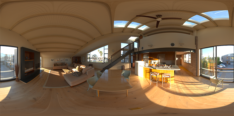
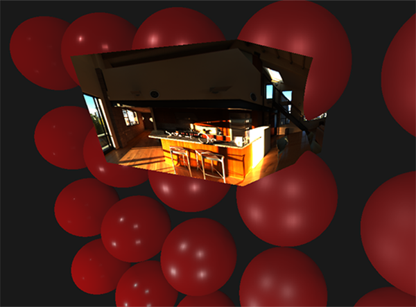
Now rendering the sampled environment map over the previously rendered spheres should look something like this:

Well... it took us quite a bit of setup to get here, but we successfully managed to read an HDR environment map, convert it from its equirectangular mapping to a cubemap and render the HDR cubemap into the scene as a skybox. Furthermore, we set up a small system to render onto all 6 faces of a cubemap which we'll need again when convoluting the environment map. You can find the source code of the entire conversion process here.

Cubemap convolution

As described at the start of the tutorial, our main goal is to solve the integral for all diffuse indirect lighting given the scene's irradiance in the form of a cubemap environment map. We know that we can get the radiance of the scene L(p,wi)L(p,wi) in a particular direction by sampling an HDR environment map in direction wiwi. To solve the integral, we have to sample the scene's radiance from all possible directions within the hemisphere ΩΩ for each fragment.

It is however computationally impossible to sample the environment's lighting from every possible direction in ΩΩ, the number of possible directions is theoretically infinite. We can however, approximate the number of directions by taking a finite number of directions or samples, spaced uniformly or taken randomly from within the hemisphere to get a fairly accurate approximation of the irradiance, effectively solving the integral ∫∫ discretely

It is however still too expensive to do this for every fragment in real-time as the number of samples still needs to be significantly large for decent results, so we want to pre-compute this. Since the orientation of the hemisphere decides where we capture the irradiance we can pre-calculate the irradiance for every possible hemisphere orientation oriented around all outgoing directions wowo:

Lo(p,ωo)=kdcπ∫ΩLi(p,ωi)n⋅ωidωiLo(p,ωo)=kdcπ∫ΩLi(p,ωi)n⋅ωidωi

Given any direction vector wiwi, we can then sample the pre-computed irradiance map to retrieve the total diffuse irradiance from direction wiwi. To determine the amount of indirect diffuse (irradiant) light at a fragment surface, we retrieve the total irradiance from the hemisphere oriented around its surface's normal. Obtaining the scene's irradiance is then as simple as:

vec3 irradiance = texture(irradianceMap, N);

Now, to generate the irradiance map we need to convolute the environment's lighting as converted to a cubemap. Given that for each fragment the surface's hemisphere is oriented along the normal vector NN, convoluting a cubemap equals calculating the total averaged radiance of each direction wiwi in the hemisphere ΩΩ oriented along NN.

Thankfully, all of the cumbersome setup in this tutorial isn't all for nothing as we can now directly take the converted cubemap, convolute it in a fragment shader and capture its result in a new cubemap using a framebuffer that renders to all 6 face directions. As we've already set this up for converting the equirectangular environment map to a cubemap, we can take the exact same approach but use a different fragment shader:

#version 330 coreout vec4 FragColor;in vec3 localPos;uniform samplerCube environmentMap;const float PI = 3.14159265359;void main(){    // the sample direction equals the hemisphere's orientation     vec3 normal = normalize(localPos);      vec3 irradiance = vec3(0.0);      [...] // convolution code      FragColor = vec4(irradiance, 1.0);}

With environmentMap being the HDR cubemap as converted from the equirectangular HDR environment map.

There are many ways to convolute the environment map, but for this tutorial we're going to generate a fixed amount of sample vectors for each cubemap texel along a hemisphere ΩΩ oriented around the sample direction and average the results. The fixed amount of sample vectors will be uniformly spread inside the hemisphere. Note that an integral is a continuous function and discretely sampling its function given a fixed amount of sample vectors will be an approximation. The more sample vectors we use, the better we approximate the integral.

The integral ∫∫ of the reflectance equation revolves around the solid angle dwdw which is rather difficult to work with. Instead of integrating over the solid angle dwdw we'll integrate over its equivalent spherical coordinates θθ and ϕϕ.

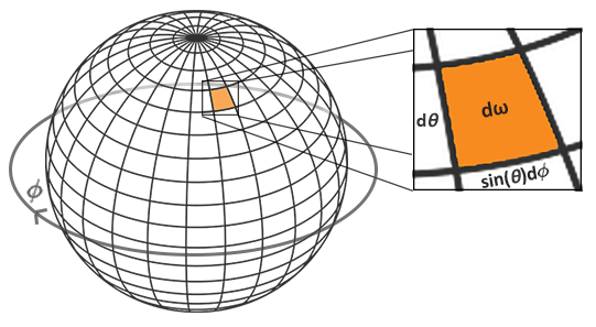
We use the polar azimuth ϕϕ angle to sample around the ring of the hemisphere between 00 and 2π2π, and use the inclination zenith θθ angle between 00 and 12π12π to sample the increasing rings of the hemisphere. This will give us the updated reflectance integral:

Lo(p,ϕo,θo)=kdcπ∫2πϕ=0∫12πθ=0Li(p,ϕi,θi)cos(θ)sin(θ)dϕdθLo(p,ϕo,θo)=kdcπ∫ϕ=02π∫θ=012πLi(p,ϕi,θi)cos⁡(θ)sin⁡(θ)dϕdθ

Solving the integral requires us to take a fixed number of discrete samples within the hemisphere ΩΩ and averaging their results. This translates the integral to the following discrete version as based on the Riemann sum given n1n1 and n2n2 discrete samples on each spherical coordinate respectively:

Lo(p,ϕo,θo)=kdcπ1n1+n2∑ϕ=0n1∑θ=0n2Li(p,ϕi,θi)cos(θ)sin(θ)dϕdθLo(p,ϕo,θo)=kdcπ1n1+n2∑ϕ=0n1∑θ=0n2Li(p,ϕi,θi)cos⁡(θ)sin⁡(θ)dϕdθ

As we sample both spherical values discretely, each sample will approximate or average an area on the hemisphere as the image above shows. Note that (due to the general properties of a spherical shape) the hemisphere's discrete sample area gets smaller the higher the zenith angle θθ as the sample regions converge towards the center top. To compensate for the smaller areas, we weigh its contribution by scaling the area by sinθsin⁡θ clarifying the added sinsin.

Discretely sampling the hemisphere given the integral's spherical coordinates for each fragment invocation translates to the following code:

vec3 irradiance = vec3(0.0);  vec3 up    = vec3(0.0, 1.0, 0.0);vec3 right = cross(up, normal);up         = cross(normal, right);float sampleDelta = 0.025;float nrSamples = 0.0; for(float phi = 0.0; phi < 2.0 * PI; phi += sampleDelta){    for(float theta = 0.0; theta < 0.5 * PI; theta += sampleDelta)    {        // spherical to cartesian (in tangent space)        vec3 tangentSample = vec3(sin(theta) * cos(phi),  sin(theta) * sin(phi), cos(theta));        // tangent space to world        vec3 sampleVec = tangentSample.x * right + tangentSample.y * up + tangentSample.z * N;         irradiance += texture(environmentMap, sampleVec).rgb * cos(theta) * sin(theta);        nrSamples++;    }}irradiance = PI * irradiance * (1.0 / float(nrSamples));

We specify a fixed sampleDelta delta value to traverse the hemisphere; decreasing or increasing the sample delta will increase or decrease the accuracy respectively.

From within both loops, we take both spherical coordinates to convert them to a 3D Cartesian sample vector, convert the sample from tangent to world space and use this sample vector to directly sample the HDR environment map. We add each sample result to irradiance which at the end we divide by the total number of samples taken, giving us the average sampled irradiance. Note that we scale the sampled color value by cos(theta) due to the light being weaker at larger angles and by sin(theta) to account for the smaller sample areas in the higher hemisphere areas.

Now what's left to do is to set up the OpenGL rendering code such that we can convolute the earlier captured envCubemap. First we create the irradiance cubemap (again, we only have to do this once before the render loop):

unsigned int irradianceMap;glGenTextures(1, &irradianceMap);glBindTexture(GL_TEXTURE_CUBE_MAP, irradianceMap);for (unsigned int i = 0; i < 6; ++i){    glTexImage2D(GL_TEXTURE_CUBE_MAP_POSITIVE_X + i, 0, GL_RGB16F, 32, 32, 0,                  GL_RGB, GL_FLOAT, nullptr);}glTexParameteri(GL_TEXTURE_CUBE_MAP, GL_TEXTURE_WRAP_S, GL_CLAMP_TO_EDGE);glTexParameteri(GL_TEXTURE_CUBE_MAP, GL_TEXTURE_WRAP_T, GL_CLAMP_TO_EDGE);glTexParameteri(GL_TEXTURE_CUBE_MAP, GL_TEXTURE_WRAP_R, GL_CLAMP_TO_EDGE);glTexParameteri(GL_TEXTURE_CUBE_MAP, GL_TEXTURE_MIN_FILTER, GL_LINEAR);glTexParameteri(GL_TEXTURE_CUBE_MAP, GL_TEXTURE_MAG_FILTER, GL_LINEAR);

As the irradiance map averages all surrounding radiance uniformly it doesn't have a lot of high frequency details so we can store the map at a low resolution (32x32) and let OpenGL's linear filtering do most of the work. Next, we re-scale the capture framebuffer to the new resolution:

glBindFramebuffer(GL_FRAMEBUFFER, captureFBO);glBindRenderbuffer(GL_RENDERBUFFER, captureRBO);glRenderbufferStorage(GL_RENDERBUFFER, GL_DEPTH_COMPONENT24, 32, 32);  

Using the convolution shader we convolute the environment map in a similar way we captured the environment cubemap:

irradianceShader.use();irradianceShader.setInt("environmentMap", 0);irradianceShader.setMat4("projection", captureProjection);glActiveTexture(GL_TEXTURE0);glBindTexture(GL_TEXTURE_CUBE_MAP, envCubemap);glViewport(0, 0, 32, 32); // don't forget to configure the viewport to the capture dimensions.glBindFramebuffer(GL_FRAMEBUFFER, captureFBO);for (unsigned int i = 0; i < 6; ++i){    irradianceShader.setMat4("view", captureViews[i]);    glFramebufferTexture2D(GL_FRAMEBUFFER, GL_COLOR_ATTACHMENT0,                            GL_TEXTURE_CUBE_MAP_POSITIVE_X + i, irradianceMap, 0);    glClear(GL_COLOR_BUFFER_BIT | GL_DEPTH_BUFFER_BIT);    renderCube();}glBindFramebuffer(GL_FRAMEBUFFER, 0);  

Now after this routine we should have a pre-computed irradiance map that we can directly use for our diffuse image based lighting. To see if we successfully convoluted the environment map let's substitute the environment map for the irradiance map as the skybox's environment sampler:

If it looks like a heavily blurred version of the environment map you've successfully convoluted the environment map.

PBR and indirect irradiance lighting

The irradiance map represents the diffuse part of the reflectance integral as accumulated from all surrounding indirect light. Seeing as the light doesn't come from any direct light sources, but from the surrounding environment we treat both the diffuse and specular indirect lighting as the ambient lighting, replacing our previously set constant term.

First, be sure to add the pre-calculated irradiance map as a cube sampler:

uniform samplerCube irradianceMap;

Given the irradiance map that holds all of the scene's indirect diffuse light, retrieving the irradiance influencing the fragment is as simple as a single texture sample given the surface's normal:

// vec3 ambient = vec3(0.03);vec3 ambient = texture(irradianceMap, N).rgb;

However, as the indirect lighting contains both a diffuse and specular part as we've seen from the split version of the reflectance equation we need to weigh the diffuse part accordingly. Similar to what we did in the previous tutorial we use the Fresnel equation to determine the surface's indirect reflectance ratio from which we derive the refractive or diffuse ratio:

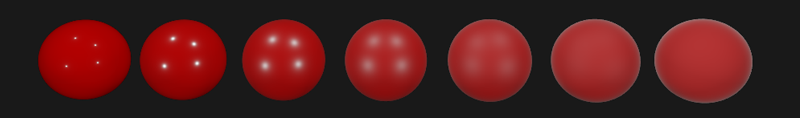
vec3 kS = fresnelSchlick(max(dot(N, V), 0.0), F0);vec3 kD = 1.0 - kS;vec3 irradiance = texture(irradianceMap, N).rgb;vec3 diffuse    = irradiance * albedo;vec3 ambient    = (kD * diffuse) * ao; 

As the ambient light comes from all directions within the hemisphere oriented around the normal N there's no single halfway vector to determine the Fresnel response. To still simulate Fresnel, we calculate the Fresnel from the angle between the normal and view vector. However, earlier we used the micro-surface halfway vector, influenced by the roughness of the surface, as input to the Fresnel equation. As we currently don't take any roughness into account, the surface's reflective ratio will always end up relatively high. Indirect light follows the same properties of direct light so we expect rougher surfaces to reflect less strongly on the surface edges. As we don't take the surface's roughness into account, the indirect Fresnel reflection strength looks off on rough non-metal surfaces (slightly exaggerated for demonstration purposes):

We can alleviate the issue by injecting a roughness term in the Fresnel-Schlick equation as described by Sébastien Lagarde:

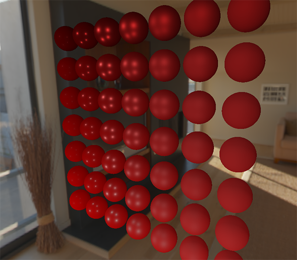
vec3 fresnelSchlickRoughness(float cosTheta, vec3 F0, float roughness){    return F0 + (max(vec3(1.0 - roughness), F0) - F0) * pow(1.0 - cosTheta, 5.0);}   

By taking account of the surface's roughness when calculating the Fresnel response, the ambient code ends up as:

vec3 kS = fresnelSchlickRoughness(max(dot(N, V), 0.0), F0, roughness); vec3 kD = 1.0 - kS;vec3 irradiance = texture(irradianceMap, N).rgb;vec3 diffuse    = irradiance * albedo;vec3 ambient    = (kD * diffuse) * ao; 

As you can see, the actual image based lighting computation is quite simple and only requires a single cubemap texture lookup; most of the work is in pre-computing or convoluting the environment map into an irradiance map.

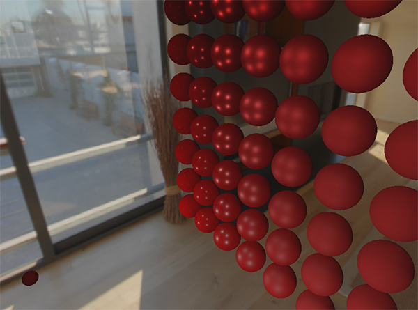
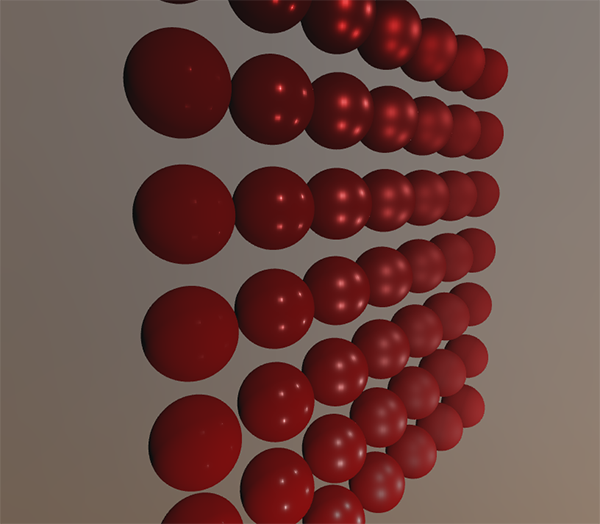
If we take the initial scene from the lighting tutorial where each sphere has a vertically increasing metallic and a horizontally increasing roughness value and add the diffuse image based lighting it'll look a bit like this:

It still looks a bit weird as the more metallic spheres require some form of reflection to properly start looking like metallic surfaces (as metallic surfaces don't reflect diffuse light) which at the moment are only coming (barely) from the point light sources. Nevertheless, you can already tell the spheres do feel more in place within the environment (especially if you switch between environment maps) as the surface response reacts accordingly to the environment's ambient lighting.

You can find the complete source code of the discussed topics here. In the next tutorial we'll add the indirect specular part of the reflectance integral at which point we're really going to see the power of PBR.

Further reading

• Coding Labs: Physically based rendering: an introduction to PBR and how and why to generate an irradiance map.
• The Mathematics of Shading: a brief introduction by ScratchAPixel on several of the mathematics described in this tutorial, specifically on polar coordinates and integrals.