My Fluid Simulation (SPH) Sample (2) – Curvature Flow

After a long time of break – break by my GI renderer, I picked up my SPH application again. In recent week, I managed to implement Curvature Flow described in the paper “Screen Space Fluid Rendering with Curvature Flow” (http://portal.acm.org/citation.cfm?id=1507149.1507164). Man it is not easy!

Here are the main steps I follow:

1. Get Depth Buffer data

Screen-space calculation is the key of the whole paper. The surface reconstruction is totally based on the depth buffer – Z-buffer in OpenGL. So the first step is to get the depth data of the particles. The popular implementation is to use Fragment shader, however I haven’t learnt it yet. So I use the slow ‘glReadPixels(GL_DEPTH_COMPONENT)’ to get it. First only particles are rendered and flushed – the first depth buffer is got; then all the other objects in the scene are rendered with depth test enabled – the second depth buffer is got. The a XOR operation is applied on the two buffers. So the screen-spaced depth information of particles can be obtained.

2. Iterative Curvature Flow

Curvature flow is an iterative process. It is just like inflating a vacuum balloon containing several particles. Yes, surface normal divergence is the key maths tool to complete this natural process. For mathematical details, please refer to the paper (as cited above). In practise, 60 – 100 iterations per frame can generate satisfactory surface reconstruction effect.

3. Surface Normal calculation

After a smoothed depth data is at hand, we need to implement rendering, so surface normals is the prerequisite for all following optical effects as reflection/refraction. Since we have already got the divergence of surface normals, the normals can be calculated using the same mathematical tool. However, because of the pixel-based essence of the depth buffer, direct applying of normals would generate serious jaggies… Interpolation is always the primary solution for jaggies.
The basic idea I use is to calculate the normals of the pixels that are on one fixed grid nodes, so all the other in-between pixel normals can be obtained using bi-linear interpolation. Care should be taken that the ‘standard’ normals on the grid nodes should be an average normal of the area around the pixel (2x2, 4x4, …) – this is a ‘democratic election’: the normal of the pixel on the grid may not represent the smoothness of the area around that pixel. This is very important because it can make the image much more similiar with the effect that it should be.

All right, screenshots:

  
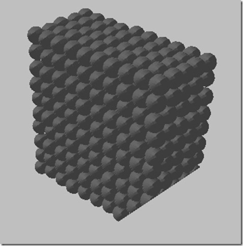
the image without Curvature Flow yet..

 
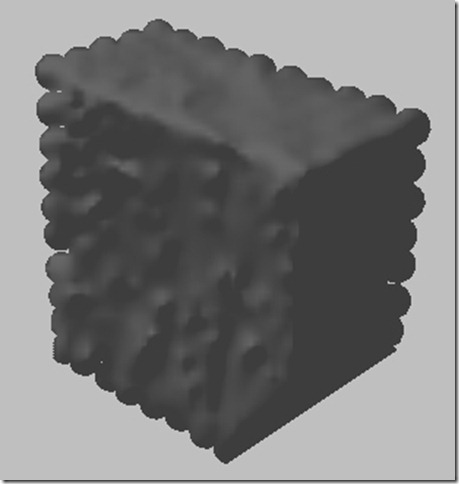
100 iterations, 4x4 average normal sampling.

See? It has been inflated! Isn’t it cool? But I know there are still artifacts from numerical dissipation, but it is already acceptable and my particles are large enough. More and smaller particles will offer a much fancier effect I believe.

TODO
1. Optical effects (Cubemap)
2. Performance tuning (CUDA, etc..)
3. Integration with physical simulation mechanism (That’ll be cool :P)

Just wait for me!