Matlab 线性拟合 & 非线性拟合
来源:互联网 发布:网络摄像机管理软件 编辑:程序博客网 时间:2024/04/26 01:22
使用Matlab进行拟合是图像处理中线条变换的一个重点内容,本文将详解Matlab中的直线拟合和曲线拟合用法。
关键函数:
fittype
Fit type for curve and surface fitting
Syntax
ffun = fittype(libname)
ffun = fittype(expr)
ffun = fittype({expr1,...,exprn})
ffun = fittype(expr, Name, Value,...)
ffun= fittype({expr1,...,exprn}, Name, Value,...)
/***********************************线性拟合***********************************/
线性拟合公式:
coeff1 * term1 + coeff2 * term2 + coeff3 * term3 + ...其中,coefficient是系数,term都是x的一次项。
线性拟合Example:
Example1: y=kx+b;
法1:
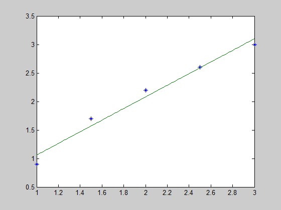
- x=[1,1.5,2,2.5,3];y=[0.9,1.7,2.2,2.6,3];
- p=polyfit(x,y,1);
- x1=linspace(min(x),max(x));
- y1=polyval(p,x1);
- plot(x,y,'*',x1,y1);
即y=1.0200 *x+ 0.0400
法2:
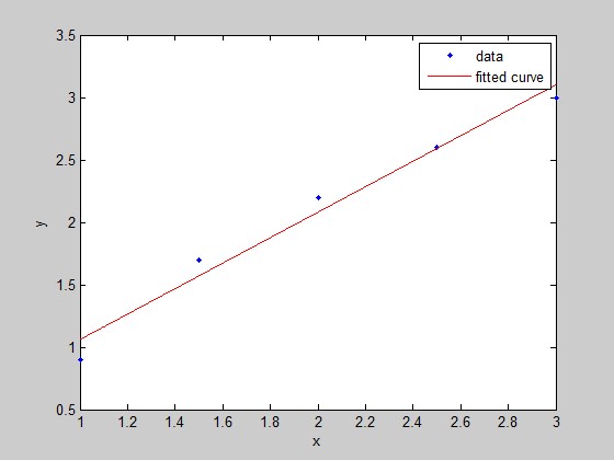
- x=[1;1.5;2;2.5;3];y=[0.9;1.7;2.2;2.6;3];
- p=fittype('poly1')
- f=fit(x,y,p)
- plot(f,x,y);
- x=[1;1.5;2;2.5;3];y=[0.9;1.7;2.2;2.6;3];
- p=fittype('poly1')
- f=fit(x,y,p)
- plot(f,x,y);
- p =
- Linear model Poly1:
- p(p1,p2,x) = p1*x + p2
- f =
- Linear model Poly1:
- f(x) = p1*x + p2
- Coefficients (with 95% confidence bounds):
- p1 = 1.02 (0.7192, 1.321)
- p2 = 0.04 (-0.5981, 0.6781)
法1:
- x=[1;1.5;2;2.5;3];y=[0.9;1.7;2.2;2.6;3];
- EXPR = {'x','sin(x)','1'};
- p=fittype(EXPR)
- f=fit(x,y,p)
- plot(f,x,y);
运行结果:
- x=[1;1.5;2;2.5;3];y=[0.9;1.7;2.2;2.6;3];
- EXPR = {'x','sin(x)','1'};
- p=fittype(EXPR)
- f=fit(x,y,p)
- plot(f,x,y);
- p =
- Linear model:
- p(a,b,c,x) = a*x + b*sin(x) + c
- f =
- Linear model:
- f(x) = a*x + b*sin(x) + c
- Coefficients (with 95% confidence bounds):
- a = 1.249 (0.9856, 1.512)
- b = 0.6357 (0.03185, 1.24)
- c = -0.8611 (-1.773, 0.05094)
法2:
- x=[1;1.5;2;2.5;3];y=[0.9;1.7;2.2;2.6;3];
- p=fittype('a*x+b*sin(x)+c','independent','x')
- f=fit(x,y,p)
- plot(f,x,y);
运行结果:
- x=[1;1.5;2;2.5;3];y=[0.9;1.7;2.2;2.6;3];
- p=fittype('a*x+b*sin(x)+c','independent','x')
- f=fit(x,y,p)
- plot(f,x,y);
- p =
- General model:
- p(a,b,c,x) = a*x+b*sin(x)+c
- Warning: Start point not provided, choosing random start
- point.
- > In fit>iCreateWarningFunction/nThrowWarning at 738
- In fit>iFit at 320
- In fit at 109
- f =
- General model:
- f(x) = a*x+b*sin(x)+c
- Coefficients (with 95% confidence bounds):
- a = 1.249 (0.9856, 1.512)
- b = 0.6357 (0.03185, 1.24)
- c = -0.8611 (-1.773, 0.05094)

/***********************************非线性拟合***********************************/
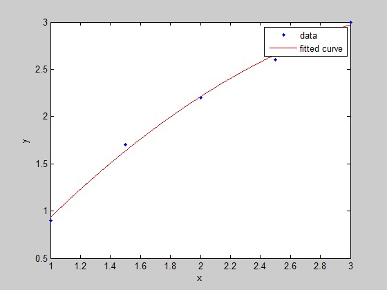
Example:y=a*x^2+b*x+c
法1:
- x=[1;1.5;2;2.5;3];y=[0.9;1.7;2.2;2.6;3];
- p=fittype('a*x.^2+b*x+c','independent','x')
- f=fit(x,y,p)
- plot(f,x,y);
运行结果:
- p =
- General model:
- p(a,b,c,x) = a*x.^2+b*x+c
- Warning: Start point not provided, choosing random start
- point.
- > In fit>iCreateWarningFunction/nThrowWarning at 738
- In fit>iFit at 320
- In fit at 109
- f =
- General model:
- f(x) = a*x.^2+b*x+c
- Coefficients (with 95% confidence bounds):
- a = -0.2571 (-0.5681, 0.05386)
- b = 2.049 (0.791, 3.306)
- c = -0.86 (-2.016, 0.2964)
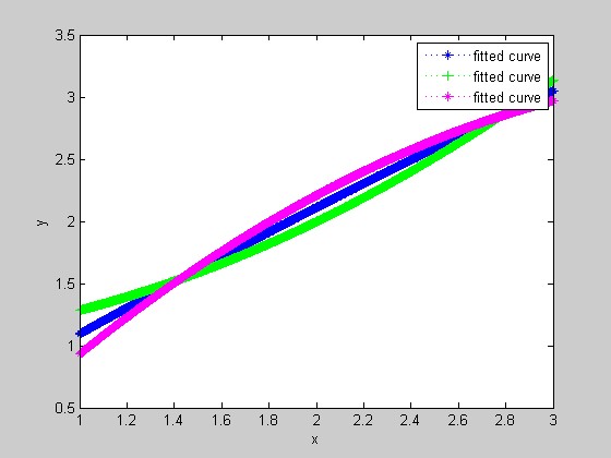
法2:
- x=[1;1.5;2;2.5;3];y=[0.9;1.7;2.2;2.6;3];
- %use c=0;
- c=0;
- p1=fittype(@(a,b,x) a*x.^2+b*x+c)
- f1=fit(x,y,p1)
- %use c=1;
- c=1;
- p2=fittype(@(a,b,x) a*x.^2+b*x+c)
- f2=fit(x,y,p2)
- %predict c
- p3=fittype(@(a,b,c,x) a*x.^2+b*x+c)
- f3=fit(x,y,p3)
- %show results
- scatter(x,y);%scatter point
- c1=plot(f1,'b:*');%blue
- hold on
- plot(f2,'g:+');%green
- hold on
- plot(f3,'m:*');%purple
- hold off
0 0
- Matlab 线性拟合 & 非线性拟合
- Matlab 线性拟合 & 非线性拟合
- Matlab 线性拟合 & 非线性拟合
- Matlab 线性拟合 & 非线性拟合
- Matlab 线性拟合 & 非线性拟合
- Matlab 线性拟合 & 非线性拟合
- Matlab 线性拟合 & 非线性拟合
- Matlab 线性拟合 & 非线性拟合
- Matlab 线性拟合 & 非线性拟合
- Matlab非线性拟合
- 关于Matlab中的线性与非线性最小二乘拟合
- 最小二乘法 线性与非线性拟合
- Matlab非线性拟合工具箱cftool
- Matlab中的lsqcurvefit,非线性拟合
- matlab线性拟合
- matlab 线性拟合
- 最小二乘法详解(线性拟合与非线性拟合)
- matlab非线性拟合所碰到的问题
- 第九周 项目六 穷举法解决组合问题4
- LUA正则表达式
- iOS UIBezierPath类 介绍
- 在服务器上部署Ubuntu
- 面向对象--组合
- Matlab 线性拟合 & 非线性拟合
- MPC制作项目文件(makefile)之一
- 注意事项
- org.springframework.beans.factory.BeanDefinitionStoreException: Unexpected exception parsing XML doc
- jquery contians(text) 选择器
- jquery ui js文件的导入顺序
- OpenCV中矩阵数据的访问(二)(Learning OpenCV第三章3)
- 11gR203RAConAix Install
- discuz ajaxpost函数解析