R语言数据分析基础

转载自：http://blog.csdn.net/simon_woo_coding/article/details/19022957

本文中使用的数据为iris(鸢尾花) 。

观察数据整体的大小与结构

> iris

   |   花萼长度     花萼宽度 花瓣长度     花瓣宽度物种 |

    Sepal.Length Sepal.Width Petal.Length Petal.Width     Species

1            5.1         3.5          1.4        0.2              setosa

2            4.9         3.0          1.4         0.2              setosa

3            4.7         3.2          1.3         0.2                 setosa

4            4.6        3.1          1.5         0.2                 setosa

5            5.0         3.6          1.4         0.2                 setosa

6            5.4         3.9          1.7         0.4                 setosa

7            4.6           3.4          1.4         0.3                 setosa

8            5.0        3.4          1.5         0.2              setosa

9            4.4         2.9          1.4         0.2              setosa

10          4.9         3.1          1.5         0.1              setosa

………

dim()返回数据的维度

> dim(iris)

|150行，5列|

[1] 150   5

names()返回数据的名称

> names(iris)

[1] "Sepal.Length" "Sepal.Width"  "Petal.Length" "Petal.Width"  "Species"

str()返回数据的整体结构

> str(iris)

'data.frame':   150 obs. of  5 variables:

$ Sepal.Length: num  5.1 4.9 4.7 4.6 5 5.4 4.6 5 4.4 4.9 ...

$ Sepal.Width : num  3.5 3 3.2 3.1 3.6 3.9 3.4 3.4 2.9 3.1 ...

$ Petal.Length: num  1.4 1.4 1.3 1.5 1.4 1.7 1.4 1.5 1.4 1.5 ...

$ Petal.Width : num  0.2 0.2 0.2 0.2 0.2 0.4 0.3 0.2 0.2 0.1 ...

$ Species     : Factor w/ 3 levels "setosa","versicolor",..: 1 1 1 1 1 1 1 1  1 1 ..

iris为data.frame类型数据，共150条数据，5个属性。

Sepal.Length为number类型数据，它的前几条属性值为....

Sepal.Width为number类型数据，它的前几条属性值为....

Petal.Length为number类型数据，它的前几条属性值为....

Petal.Width为number类型数据，它的前几条属性值为....

Species为Factor类型数据，共3个levels:setosa,versicolor,....

> attributes(iris)

$names

[1] "Sepal.Length" "Sepal.Width"  "Petal.Length" "Petal.Width"  "Species"     

$row.names

 [1]   1   2   3   4   5   6   7   8   9  10  11  12  13  14  15  16  17  18

[19]  19  20  21  22  23  24  25  26  27  28  29  30  31  32  33  34  35  36

[37]  37  38  39  40  41  42  43  44  45  46  47  48  49  50  51  52  53  54

[55]  55  56  57  58  59  60  61  62  63  64  65  66  67  68  69  70  71  72

[73]  73  74  75  76  77  78  79  80  81  82  83  84  85  86  87  88  89  90

[91]  91  92  93  94  95  96  97  98  99 100 101 102 103 104 105 106 107 108

[109] 109 110 111 112 113 114 115 116 117 118 119 120 121 122 123 124 125 126

[127] 127 128 129 130 131 132 133 134 135 136 137 138 139 140 141 142 143 144

[145] 145 146 147 148 149 150

$class

[1] "data.frame"

attributes返回数据的整体属性

names为数据属性的名称

row.names为每条数据的名称

class为数据结构类型

head()返回数据集的前几条数据

tail()返回数据集的后几条数据

> head(iris)

 Sepal.Length Sepal.Width Petal.Length Petal.Width Species

1          5.1         3.5          1.4         0.2 setosa

2          4.9         3.0          1.4         0.2  setosa

3          4.7         3.2          1.3         0.2  setosa

4          4.6         3.1          1.5         0.2  setosa

5          5.0         3.6          1.4         0.2  setosa

6          5.4         3.9          1.7         0.4  setosa

与我们观察到的iris数据一致。

观察单条数据的属性

> summary(iris)

 Sepal.Length    Sepal.Width     Petal.Length    Petal.Width   

Min.   :4.300   Min.   :2.000   Min.   :1.000   Min.   :0.100  

1st Qu.:5.100   1st Qu.:2.800   1st Qu.:1.600   1st Qu.:0.300  

Median :5.800   Median :3.000   Median :4.350   Median :1.300  

Mean   :5.843   Mean   :3.057   Mean   :3.758   Mean   :1.199  

3rd Qu.:6.400   3rd Qu.:3.300   3rd Qu.:5.100   3rd Qu.:1.800  

Max.   :7.900   Max.   :4.400   Max.   :6.900   Max.   :2.500  

      Species  

setosa    :50  

versicolor:50  

virginica :50

summary()返回每个属性中最小值，最大值，中值，平均值，四分之一值，四分之三值。

对于factor类型返回每个level的比例。

> var(iris$Sepal.Width)

[1] 0.1899794

var()返回方差。

> hist(iris$Sepal.Length)

hist返回数据的分布图。

> plot(density(iris$Sepal.Length))

density返回数据的密度图。

> table(iris$Species)

   setosa versicolor  virginica

       50         50         50

table返回factor类型各种level的分布。

> pie(table(iris$Species)

> barplot(table(iris$Species))

观察多重数据间的关系

cov()返回方差

> cov(iris$Sepal.Length, iris$Petal.Length)

[1] 1.274315

> cov(iris[,1:4])

Sepal.Length Sepal.Width Petal.Length Petal.Width

Sepal.Length 0.6856935 -0.0424340 1.2743154 0.5162707

Sepal.Width -0.0424340 0.1899794 -0.3296564 -0.1216394

Petal.Length 1.2743154 -0.3296564 3.1162779 1.2956094

Petal.Width 0.5162707 -0.1216394 1.2956094 0.5810063

cor()返回协方差。

> cor(iris$Sepal.Length, iris$Petal.Length)

[1] 0.8717538

> cor(iris[,1:4])

Sepal.Length Sepal.Width Petal.Length Petal.Width

Sepal.Length 1.0000000 -0.1175698 0.8717538 0.8179411

Sepal.Width -0.1175698 1.0000000 -0.4284401 -0.3661259

Petal.Length 0.8717538 -0.4284401 1.0000000 0.9628654

Petal.Width 0.8179411 -0.3661259 0.9628654 1.0000000

> aggregate(Sepal.Length ~ Species, summary, data=iris)

Species Sepal.Length.Min. Sepal.Length.1st Qu. Sepal.Length.Median

1 setosa4.3004.8005.000

2 versicolor4.9005.6005.900

3 virginica4.9006.2256.500

Sepal.Length.Mean Sepal.Length.3rd Qu. Sepal.Length.Max.

15.0065.2005.800

25.9366.3007.000

36.5886.9007.900

> boxplot(Sepal.Length~Species, data=iris)

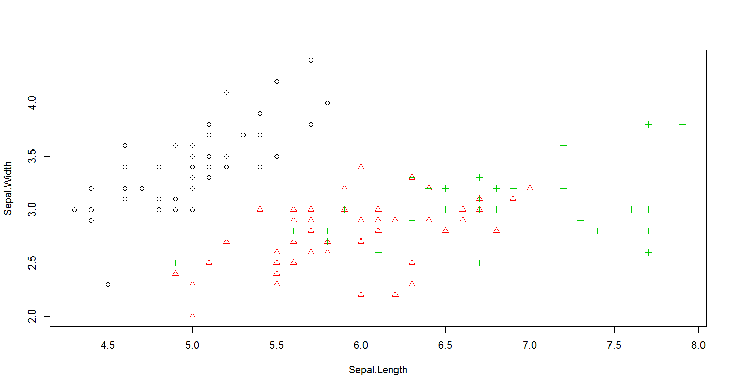
with(iris, plot(Sepal.Length, Sepal.Width, col=Species, pch=as.numeric(Species)))

with(iris, plot(Petal.Length, Petal.Width, col=Species, pch=as.numeric(Species)))