Article - Physically Based Rendering

Introduction

The pursuit of realism is pushing rendering technology towards a detailed simulation of how light works and interacts with objects. Physically based rendering is a catch all term for any technique that tries to achieve photorealism via physical simulation of light.

Currently the best model to simulate light is captured by an equation known as the rendering equation. The rendering equation tries to describe how a "unit" of light is obtained given all the incoming light that interacts with a specific point of a given scene. We will see the details and introduce the correct terminology in a moment. It's important to notice that we won't try to solve thefull rendering equation, instead we will use the following simplified version:

Lo(p,ωo)=∫Ωfr(p,ωi,ωo)Li(p,ωi)n⋅ωidωiLo(p,ωo)=∫Ωfr(p,ωi,ωo)Li(p,ωi)n⋅ωidωi

To understand this equation we first need to understand how the light works, and then, we will need to agree on some common terms. To give you a rough idea of what the formula means, in simple terms, we could say that the formula describes the colour of a pixel given all the incoming 'coloured light' and a function that tells us how to mix them.

Physics terms

If we want to properly understand the rendering equation we need to capture the meaning of some physical quantities; the most important of these quantities is called radiance (represented with LL in the formula). 
Radiance is a tricky thing to understand, as it is a combination of other physics quantities, therefore, before formally define it, we will introduce a few other quantities.

Radiant Flux: The radiant flux is the measure of the total amount of energy, emitted by a light source, expressed in Watts. We will represent the flux with the Greek letter ΦΦ. 
Any light source emits energy, and the amount of emitted energy is function of the wavelength. 

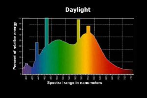Figure 1: Daylight spectral distribution

In figure 1 we can see the spectral distribution for day light; the radiant flux is the area of the function (to be exact, the area is the luminous flux, as the graph is limiting the wavelength to the human visible spectrum). For our purposes we will simplify the radiant flux with an RGB colour, even if this means losing a lot of information. 

Solid angle: It's a way to measure how large an object appears to an observer looking from a point. To do this we project the silhouette of the object onto the surface of a unit sphere centred in the point we are observing from. The area of the shape we have obtained is the solid angle. In Figure 2 you can see the solid angle ωω as a projection of the light blue polygon on the unit sphere.

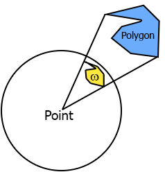Figure 2: Solid angle
 

Radiant Intensity: is the amount of flux per solid angle. If you have a light source that emits in all directions, how much of that light (flux) is actually going towards a specific direction? Intensity is the way to answer to that, it's the amount of flux that is going in one direction passing through a defined solid angle. The formula that describes it is I=dΦdωI=dΦdω, where ΦΦ is the radiant flux and ωω is the solid angle.

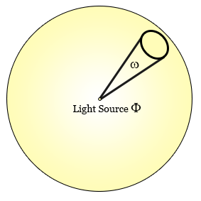Figure 3: Light intensity

Radiance: finally, we get to radiance. Radiance formula is:

L=dϕ2dAdωcosθL=dϕ2dAdωcosθ

where ΦΦ is the radiant flux, AA is the area affected by the light, ωω is the solid angle where the light is passing through and cosθcosθ is a scaling factor that "fades" the light with the angle. 

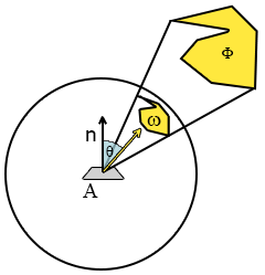Figure 4: Radiance components
 

We like this formula because it contains all the physical components we are interested in, and we can use it to describe a single"ray" of light. In fact we can use radiance to describe the amount of flux, passing through an infinitely small solid angle, hitting an infinitely small area, and that describes the behaviour of a light ray. So when we talk about radiance we talk about some amount of light going in some direction to some area.
When we shade a point we are interested in all the incoming light into that point, that is the sum of all the radiance that hit a hemisphere centred on the point itself; the name for this entity is irradiance. Irradiance and radiance are our main physical quantities, and we will work on both of them to achieve our physically based rendering.

The rendering equation

We can now go back on the rendering equation and try to fully understand it.

Lo(p,ωo)=∫Ωfr(p,ωi,ωo)Li(p,ωi)n⋅ωidωiLo(p,ωo)=∫Ωfr(p,ωi,ωo)Li(p,ωi)n⋅ωidωi

 

We know understand  that LL is radiance, and it's function of some point in the world and some direction plus the solid angle (we will always use infinitely small solid angles from now on, so think of it simply as a direction vector). The equation describes the outgoing radiance from a point Lo(p,ωo)Lo(p,ωo), which is all we need to colour a pixel on screen.

To calculate it we need the normal of the surface where our pixel lies on (nn), and the irradiance of the scene, which is given by  Li(p,ωi)∀ωiLi(p,ωi)∀ωi. To obtain the irradiance we sum them all the incoming radiance, hence the integral sign in front of the equation. Note that the domain of the integral ΩΩ is a semi-sphere centered at the point we are calculating and oriented so that the top of the hemisphere itself can be found by moving away from the point along the normal direction.

 

The dot product n⋅ωin⋅ωi is there to take into account the angle of incidence angle of the light ray. If the ray is perpendicular to the surface it will be more localized on the lit area, while if the angle is shallow it will be spread across a bigger area, eventually spreading across too much to actually being visible.

 

Now we can see that the equation is simply representing the outgoing radiance given the incoming radiance weighted by the cosine of the angle between every incoming ray and the normal to the surface. The only bit we still need to introduce is fr(p,ωi,ωo)fr(p,ωi,ωo), that is the BRDF. This function takes as input position, incoming and outgoing ray, and outputs a weight of how much the incoming ray is contributing to the final outgoing radiance. For a perfectly specular reflection, like a mirror, the BRDF function is 0 for every incoming ray apart for the one that has the same angle of the outgoing ray, in which case the function returns 1 (the angle is measured between the rays and the surface normal). It's important to notice that a physically based BRDF has to respect the law of conservation of energy, that is ∀ωi∫Ωfr(p,ωi,ωo)(n⋅ωi)dωo≤1∀ωi∫Ωfr(p,ωi,ωo)(n⋅ωi)dωo≤1, which means that she sum of reflected light must not exceed the amount of incoming light.

 

Translate to code

So, now that we have all this useful knowledge, how do we apply it to actually write something that renders to the screen? We have two main problems here.

• First of all, how can we represent all these radiance functions in the scene?
• And secondly, how do we solve the integral fast enough to be able to use this in a real-time engine?

The answer to the first question is simple, environment maps. For our purposes we'll use environment maps (cubemaps, although spherical maps would be more suited) to encode the incoming radiance from a specific direction towards a given point. 
If we imagine that every pixel of the cubemap is a small emitter whose flux is the RGB colour, we can approximate
L(p,ω)L(p,ω), with p being the exact center of the cubemap, to a texture read from the cubemap itself, so L(p,ω)≈texCUBE(cubemap,ω)L(p,ω)≈texCUBE(cubemap,ω). Obviously it would be too much memory consuming to have a cubemap for every point in the scene(!), therefore we trade off some quality by creating a certain number of cubemaps in the scene and  every point picks the closest one. To reduce the error we can correct the sampling vector with the world position of the cubemap to be more accurate. This gives us a way to evaluate radiance, which is:

L(p,ω)=texCUBE(cubemap,ωp)L(p,ω)=texCUBE(cubemap,ωp)

where ωpωp is the sampling vector corrected by the point position and cubemap position in the world.

The answer for our second problem, how to solve the integral, is a bit more tricky, because in some cases, we won't be able to solve it quickly enough. But if the BRDF happens to depend only on the incoming radiance, or even better, on nothing (if it's constant), then we can do some nice optimization. So let's see how this happens if we plug in Lambert's BRDF, which is a constant factor (all the incoming radiance contributes to the outgoing ray after being scaled by a constant).

Lambert

Lambert's BRDF sets fr(p,ωi,ωo)=cπfr(p,ωi,ωo)=cπ where cc is the surface colour. If we plug this into the rendering equation we get:

Lo(p,ωo)=∫ΩcπLi(p,ωi)(n⋅ωi)dωi=Lo(p,ωo)=∫ΩcπLi(p,ωi)(n⋅ωi)dωi=

Lo(p,ωo)=cπ∫ΩLi(p,ωi)(n⋅ωi)dωiLo(p,ωo)=cπ∫ΩLi(p,ωi)(n⋅ωi)dωi

 

Now, the integral depends on ωiωi and nothing else, which means we can precalculate it (solving it with a Monte Carlo integration for example) and store the result into another cubemap. The value will be stored in ωoωo direction, which means that knowing what output direction we have we can sample the cubemap and obtain the reflected light in that very direction. This reduces the whole rendering equation to a single sample from a pre-calculated cubemap, specifically:

L(p,ωo)=texCUBE(lambertCubemap,ωop)L(p,ωo)=texCUBE(lambertCubemap,ωop)

 

where ωopωop is the outgoing radiance corrected by the point position and cubemap position in the world.
So, now we have all the elements, and we can finally write a shader. I'll show that in a moment, but for now, let's see the results.
 

 

Quite good for a single texture read shader uh? Please note how the whole lighting changes with the change of the envinroment (the cubemap rendered is not the convolved one, which looks way more blurry as shown below).

 

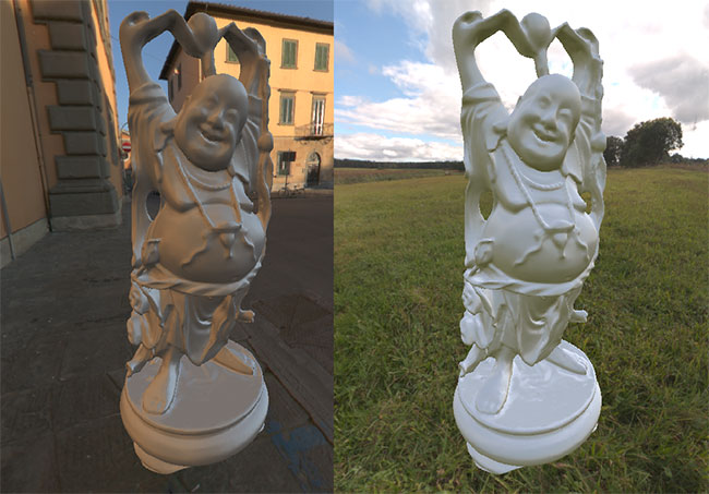
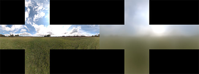Figure 5: Left the radiance map, right the irradiance map (Lambert rendering equation)
 

 

Now let's present the shader's code. Please note that for simplicity I'm not using the Monte Carlo integration but I've simply discretized the integral. Given infinite samples it wouldn't make any difference, but in a real case it will introduce more banding than Monte Carlo. In my tests it was good enough given that I've dropped the resolution of the cubemap to a 32x32 per face, but it's worth bearing this in mind if you want to experiment with it.

The first shader we need is the one that generates the blurry envmap (often referred to as the convolved envmap, since it is the result of the convolution of the radiance envmap and the kernel function (n⋅ωi)(n⋅ωi) ).

Since in the shader we will integrate in spherical coordinates we will change the formula to reflect that.

Lo(p,θo,ϕo)=cπ∫Φ∫ΘLi(p,θi,ϕi)cos(θi)sin(θi)dθidϕiLo(p,θo,ϕo)=cπ∫Φ∫ΘLi(p,θi,ϕi)cos(θi)sin(θi)dθidϕi

 

You may have noticed that there is an extra sin(θi)sin(θi) in the formula; that is due to the fact that the integration is made of small uniform steps. When we are using the solid angle this is fine as the solid angles are evenly distributed on the integration area, but when we change to spherical coordinates we will get more samples where θθ is zero and less where it goes to π2π2. If you create a sphere in your favorite modeling tool and check it's wireframe you'll see what I mean. The sin(θi)sin(θi) function is there to compensate the distribution as dωi=sin(θ)dθdϕdωi=sin⁡(θ)dθdϕ.

The double integral is solved by applying a Monte Carlo estimator on each one; this leads to the following discrete equation that we can finally transform into shader code:

Lo(p,θo,ϕo)=cπ2πN1π2N2∑N1∑N2Li(p,θi,ϕi)cos(θi)sin(θi)Lo(p,θo,ϕo)=cπ2πN1π2N2∑N1∑N2Li(p,θi,ϕi)cos(θi)sin(θi)

Lo(p,θo,ϕo)=πcN1N2∑N1∑N2Li(p,θi,ϕi)cos(θi)sin(θi)Lo(p,θo,ϕo)=πcN1N2∑N1∑N2Li(p,θi,ϕi)cos(θi)sin(θi)

...float4 PixelShaderFunction(VertexShaderOutput input) : COLOR{    float3 normal = normalize( float3(input.InterpolatedPosition.xy, 1) );    if(cubeFace==2)        normal = normalize( float3(input.InterpolatedPosition.x,  1, -input.InterpolatedPosition.y) );    else if(cubeFace==3)        normal = normalize( float3(input.InterpolatedPosition.x, -1,  input.InterpolatedPosition.y) );    else if(cubeFace==0)        normal = normalize( float3(  1, input.InterpolatedPosition.y,-input.InterpolatedPosition.x) );    else if(cubeFace==1)        normal = normalize( float3( -1, input.InterpolatedPosition.y, input.InterpolatedPosition.x) );    else if(cubeFace==5)        normal = normalize( float3(-input.InterpolatedPosition.x, input.InterpolatedPosition.y, -1) );    float3 up = float3(0,1,0);    float3 right = normalize(cross(up,normal));    up = cross(normal,right);    float3 sampledColour = float3(0,0,0);    float index = 0;    for(float phi = 0; phi < 6.283; phi += 0.025)    {        for(float theta = 0; theta < 1.57; theta += 0.1)        {            float3 temp = cos(phi) * right + sin(phi) * up;            float3 sampleVector = cos(theta) * normal + sin(theta) * temp;            sampledColour += texCUBE( diffuseCubemap_Sampler, sampleVector ).rgb *                                       cos(theta) * sin(theta);            index ++;        }    }    return float4( PI * sampledColour / index), 1 );}...

I've omitted the vertex shader and the variables definition and the source shader I've used is in HLSL. Running this for every face of the convolved cubemap using the normal cubemap as input gives us the irradiance map. We can now use the irradiance map as an input for the next shader, the model shader.

...float4 PixelShaderFunction(VertexShaderOutput input) : COLOR{    float3 irradiance= texCUBE(irradianceCubemap_Sampler, input.SampleDir).rgb;    float3 diffuse = materialColour * irradiance;    return float4( diffuse , 1); }...

Very short and super fast to evaluate.
This concludes the first part of the article on physically based rendering. I'm planning to write a second part on how to implement a more interesting BRDF like Cook-Torrance's BRDF.