BP神经网络的MATLAB实现

---

算法流程

关于BP神经网络的公式推导，上一篇博文《BP神经网络原理简单介绍以及公式推导（矩阵形式和分量形式） 》已经做了详细的说明。接下来，我们利用MATLAB对BP神经网络进行实现。我们直接上代码，并进行解释。

MATLAB 代码

整个代码是基于BP神经网络矩阵形式编写的，对公式有疑惑的同学可以参考下上篇博文。

sigmoid.m

function [ out ] = sigmoid( in )%SIGMOID Summary of this function goes here%   Detailed explanation goes here    out = 1./(1+exp(-in));end

。Sigmoid的函数一般形式有：

f(x)=11+e−2λx，f′(x)=2λf(x)(1−f(x))f(x)=1−e−2λx1−e−2λx,f′(x)=λ(1−f2(x))

它们导数都是自相关的。我们的激活函数就选择最简单的Sigmoid的函数，f(x)=11+e−x，其导数为：f′(x)=f(x)(1−f(x))

create_w.m

function [ W ] = create_w( n_levels )%CREATE_W Summary of this function goes here%   Detailed explanation goes here    n_level = numel(n_levels) - 1;    W = cell(n_level,1);    for i=1:n_level       W{i} = ones(n_levels(i+1), n_levels(i));     endend

创建权值矩阵，初始值都是1。其中n_levels是一个向量，描述了神经网络的结构，比如

n_levels = [2 6 1]

描述了一个2-6-1的网络，也就是输入层2个神经元，隐藏层6个神经元，输出层1个神经元。上篇推导公式博文中的网络可以被描述为6-4-2-2网络。
每一层的权值矩阵与上一层的输入个数和这一层的输出个数有关。

create_theta.m

function [ theta ] = create_theta( levels )%CREATE_THETA Summary of this function goes here%   Detailed explanation goes here    n_level = numel(levels) - 1;    theta = cell(n_level, 1);    for i=1:n_level       theta{i} = ones(levels(i+1),1);     endend

创建偏移量矩阵，初始值为1。

BP_predict.m

function [ output, Y ] = BP_predict( input, W, theta)%BP_ Summary of this function goes here%   Detailed explanation goes here    f = @sigmoid;    n_w = numel(W);    Y = cell(n_w+1, 1);    Y{1} = input';    for i=1:n_w        net = W{i}*Y{i} + theta{i};        Y{i+1} = f(net);    end    output = Y{end};end

在训练中，需要对目前的W和theta是否符合要求，因此需要进行预测。BP_predict是专门为了训练写的预测函数，只能对单个数据，返回值包括了中间层的输出Y。

BP_predict2.m

function [ output] = BP_predict2( input, W, theta)%BP_ Summary of this function goes here%   Detailed explanation goes here    f = @sigmoid;    n_w = numel(W);    y = input';    for i=1:n_w        net = bsxfun(@plus,W{i}*y,theta{i});        y = f(net);    end    output = y;end

BP_predict2用于预测，可以对一个数据矩阵进行预测。

BP_tranning.m

function [ W,theta ] = BP_tranning( X, levels, step )%BP_TRANNING Summary of this function goes here%   Detailed explanation goes here    if nargin < 3       step = 0.001;     end    n_levels = size(levels, 2) - 1;    n_input = levels(1);    W = create_w(levels);    theta = create_theta(levels);    [n_data,col] = size(X);    n_label = col - n_input;    tranning_data = X(:,1:n_input); %Y0 is input    label = X(:,n_input+1:end)';    f = @sigmoid;    eps = 10e-7;    old_error = 0;    while true        for k=1:n_data           [output, Y] =  BP_predict(tranning_data(k,:), W, theta);           delta = label(:,k) - output;           % update the W, from the last layer to the first layer           for l=n_levels:-1:1              net = W{l}*Y{l} + theta{l};              if l == n_levels                  S = diag(f(net).*(1-f(net)))*delta;              else                  S = diag((f(net).*(1-f(net))))*W{l+1}'*S;              end              %dW = -S*Y{l}';              new_W{l} = W{l} + step*S*Y{l}';              new_theta{l} = theta{l} + step*S;           end % end update           W = new_W;           theta = new_theta;        end % end for        y = BP_predict2(tranning_data, W, theta);        delta = y - label;        error = sum(sum(delta.^2));        if abs(error - old_error) < eps;            break;        else            old_error = error;        end    endend

训练的中止条件，个人觉得很难确定。不得已，写了一个不那么合理的：就是通过比较前后两次的错误率，错误率变化很小很小，说明错误率很难降低了，模型趋于稳定了。
其中Y{l}，对应公式中的Y(l−1)，因为MATLAB中下标从1开始。

测试

demo_3class.m

%% Build a tranning set of three classc_1 = [0 0];c_2 = [0 1];c_3 = [1 0];c_4 = [1 1];n_L1 = 20; % number of label 1n_L2 = 20; % number of label 2n_L3 = 20; % number of label 3A = zeros(n_L1, 4);A(:,3) = 0; A(:,4) = 0;for i=1:n_L1    A(i,1:2) = c_1 + rand(1,2)/2;endB = zeros(n_L2, 4);B(:,3) = 0; B(:,4) = 1;for i=1:n_L2    B(i,1:2) = c_2 + rand(1,2)/2;endC = zeros(n_L3, 4);C(:,3) = 1; C(:,4) = 0;for i=1:n_L3    C(i,1:2) = c_3 + rand(1,2)/2;endD = zeros(n_L3, 4);D(:,3) = 1; D(:,4) = 0;for i=1:n_L3    D(i,1:2) = c_4 + rand(1,2)/2;endscatter(A(:,1), A(:,2),[],'r');hold onscatter(B(:,1), B(:,2),[],'g');hold onscatter(C(:,1), C(:,2),[],'k');hold onscatter(D(:,1), D(:,2),[],'k');X = [A;B;C;D];%% Trainning the BP networkdbstop if errorn_label = 2;% create the weight matrixn_input = size(X,2) - n_label;% number of feature of each data, here is 2, only x-axis and y-axislevels = [n_input 7 n_label];step = 0.1;[W,theta] = BP_tranning(X, levels, step);save three_class W theta%% show the resultinput = X(:,1:n_input);label = X(:,n_input+1:end);y = BP_predict2(input, W, theta);Y = y';Y(find(Y>0.5)) = 1;Y(find(Y<=0.5)) = 0;T = sum(label - Y, 2);error_index = find(T ~= 0);figure;scatter(X(:,1), X(:,2), [], 'g');hold onscatter(X(error_index,1), X(error_index,2), [], 'r');

演示了一个三类分类器。对于多类分类，神经网络应该有多个输出，每个输出为0或者1，组合得到结果。比如这个例子，00表示第一类，01表示第二类，10表示第三类。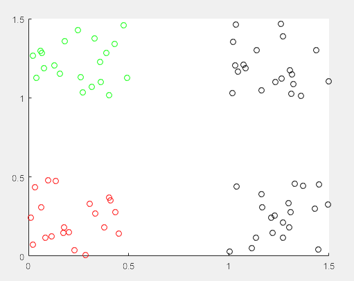

上图是初始训练数据，每种颜色代表一类。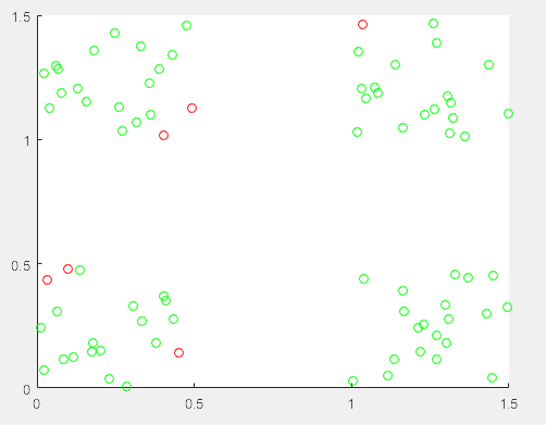

上图是训练之后，对训练集进行预测的结果，其中红色表示错误，绿色表示正确。

总结

整体来说，实现BP算法不难，但是在实验部分却发现模型的选择、step的选择、终止条件的选择都很麻烦。已经隐约感受到调参民工的辛苦了。所有代码可以在这里下载