逻辑回归softmax神经网络实现手写数字识别(cs)

逻辑回归softmax神经网络实现手写数字识别全过程

项目已上传至github：marsggbo/MLinAction

---

1 - 导入模块

import numpy as npimport matplotlib.pyplot as pltfrom ld_mnist import load_digits%matplotlib inline

2 - 导入数据及数据预处理

mnist = load_digits()

Extracting C:/Users/marsggbo/Documents/Code/ML/TF Tutorial/data/MNIST_data\train-images-idx3-ubyte.gzExtracting C:/Users/marsggbo/Documents/Code/ML/TF Tutorial/data/MNIST_data\train-labels-idx1-ubyte.gzExtracting C:/Users/marsggbo/Documents/Code/ML/TF Tutorial/data/MNIST_data\t10k-images-idx3-ubyte.gzExtracting C:/Users/marsggbo/Documents/Code/ML/TF Tutorial/data/MNIST_data\t10k-labels-idx1-ubyte.gz

print("Train: "+ str(mnist.train.images.shape))print("Train: "+ str(mnist.train.labels.shape))print("Test: "+ str(mnist.test.images.shape))print("Test: "+ str(mnist.test.labels.shape))

Train: (55000, 784)Train: (55000, 10)Test: (10000, 784)Test: (10000, 10)

mnist数据采用的是TensorFlow的一个函数进行读取的，由上面的结果可以知道训练集数据X_train有55000个，每个X的数据长度是784（28*28）。

另外由于数据集的数量较多，所以TensorFlow提供了批量提取数据的方法，从而大大提高了运行速率，方法如下：

x_batch, y_batch = mnist.train.next_batch(100)print(x_batch.shape)print(y_batch.shape)>>>(100, 784)(100, 10)

x_train, y_train, x_test, y_test = mnist.train.images, mnist.train.labels, mnist.test.images, mnist.test.labels

因为训练集的数据太大，所以可以再划分成训练集，验证集，测试集，比例为6:2:2

x_train_batch, y_train_batch = mnist.train.next_batch(30000)x_cv_batch, y_cv_batch = mnist.train.next_batch(15000)x_test_batch, y_test_batch = mnist.train.next_batch(10000)print(x_train_batch.shape)print(y_cv_batch.shape)print(y_test_batch.shape)

(30000, 784)(15000, 10)(10000, 10)

展示手写数字

nums = 6for i in range(1,nums+1):    plt.subplot(1,nums,i)    plt.imshow(x_train[i].reshape(28,28), cmap="gray")

3 - 算法介绍

3.1 算法

对单个样本数据 x(i):

z(i)=wTx(i)+b(1)

y^(i)=a(i)=softmax(z(i))(2)

损失函数

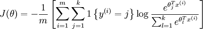
训练数据集总的损失函数表达式

需要注意的是公式(1)中的wTx(i)，这个需要视情况而定,因为需要根据数据维度的不同而进行改变。例如在本次项目中，x∈R55000×784,w∈R784×10,y∈R55000×10，所以z(i)=x(i)w+b

关键步骤
- 初始化模型参数
- 使用参数最小化cost function
- 使用学习得到的参数进行预测
- 分析结果和总结

3.2 初始化模型参数

# 初始化模型参数def init_params(dim1, dim2):    '''    dim: 表示权重w的个数，一般来说w维度要与样本x_train.shape[1]和y_train.shape[1]相匹配    '''    w = np.zeros((dim1,dim2))    return w

w  = init_params(2,1)print(w)

[[ 0.] [ 0.]]

3.3 定义softmax函数

参考Python - softmax 实现

def softmax(x):    """    Compute the softmax function for each row of the input x.    Arguments:    x -- A N dimensional vector or M x N dimensional numpy matrix.    Return:    x -- You are allowed to modify x in-place    """    orig_shape = x.shape    if len(x.shape) > 1:        # Matrix        exp_minmax = lambda x: np.exp(x - np.max(x))        denom = lambda x: 1.0 / np.sum(x)        x = np.apply_along_axis(exp_minmax,1,x)        denominator = np.apply_along_axis(denom,1,x)         if len(denominator.shape) == 1:            denominator = denominator.reshape((denominator.shape[0],1))        x = x * denominator    else:        # Vector        x_max = np.max(x)        x = x - x_max        numerator = np.exp(x)        denominator =  1.0 / np.sum(numerator)        x = numerator.dot(denominator)    assert x.shape == orig_shape    return x

a = np.array([[1,2,3,4],[1,2,3,4]])print(softmax(a))np.sum(softmax(a))

[[ 0.0320586   0.08714432  0.23688282  0.64391426] [ 0.0320586   0.08714432  0.23688282  0.64391426]]2.0

3.4 - 前向&反向传播(Forward and Backward propagation)

参数初始化后，可以开始实现FP和BP算法来让参数自学习了。

Forward Propagation:
- 获取数据X
- 计算 A=softmax(wTX+b)=(a(0),a(1),...,a(m−1),a(m))
- 计算 cost function:

def propagation(w, c, X, Y):    '''    前向传播    '''    m = X.shape[0]    A = softmax(np.dot(X,w))    J  = -1/m * np.sum(Y*np.log(A)) + 0.5*c*np.sum(w*w)    dw = -1/m * np.dot(X.T, (Y-A)) + c*w    update = {"dw":dw, "cost": J}    return update

def optimization(w, c, X, Y, learning_rate=0.1, iterations=1000, print_info=False):    '''    反向优化    '''    costs = []    for i in range(iterations):        update = propagation(w, c, X, Y)        w -= learning_rate * update['dw']        if i %100==0:            costs.append(update['cost'])        if i%100==0 and print_info==True:            print("Iteration " + str(i+1) + " Cost = " + str(update['cost']))    results = {'w':w, 'costs': costs}    return results

def predict(w, X):    '''    预测    '''    return softmax(np.dot(X, w))

def accuracy(y_hat, Y):    '''    统计准确率    '''    max_index = np.argmax(y_hat, axis=1)    y_hat[np.arange(y_hat.shape[0]), max_index] = 1    accuracy = np.sum(np.argmax(y_hat, axis=1)==np.argmax(Y, axis=1))       accuracy = accuracy *1.0/Y.shape[0]    return accuracy

def model(w, c, X, Y, learning_rate=0.1, iterations=1000, print_info=False):    results = optimization(w, c, X, Y, learning_rate, iterations, print_info)    w = results['w']    costs = results['costs']    y_hat = predict(w, X)    accuracy = accuracy(y_hat, Y)    print("After %d iterations,the total accuracy is %f"%(iterations, accuracy))    results = {        'w':w,        'costs':costs,        'accuracy':accuracy,        'iterations':iterations,        'learning_rate':learning_rate,        'y_hat':y_hat,        'c':c    }    return results

4 - 验证模型

w = init_params(x_train_batch.shape[1], y_train_batch.shape[1])c = 0results_train = model(w, c, x_train_batch, y_train_batch, learning_rate=0.3, iterations=1000, print_info=True)print(results_train)

Iteration 1 Cost = 2.30258509299Iteration 101 Cost = 0.444039646187Iteration 201 Cost = 0.383446527394Iteration 301 Cost = 0.357022940232Iteration 401 Cost = 0.341184601147Iteration 501 Cost = 0.330260258921Iteration 601 Cost = 0.322097106964Iteration 701 Cost = 0.315671301537Iteration 801 Cost = 0.310423971361Iteration 901 Cost = 0.306020145234After 1000 iterations,the total accuracy is 0.915800{'w': array([[ 0.,  0.,  0., ...,  0.,  0.,  0.],       [ 0.,  0.,  0., ...,  0.,  0.,  0.],       [ 0.,  0.,  0., ...,  0.,  0.,  0.],       ...,        [ 0.,  0.,  0., ...,  0.,  0.,  0.],       [ 0.,  0.,  0., ...,  0.,  0.,  0.],       [ 0.,  0.,  0., ...,  0.,  0.,  0.]]), 'costs': [2.302585092994045, 0.44403964618714781, 0.38344652739376933, 0.35702294023246306, 0.34118460114650634, 0.33026025892089478, 0.32209710696427363, 0.31567130153696982, 0.31042397136133199, 0.30602014523405535], 'accuracy': 0.91579999999999995, 'iterations': 1000, 'learning_rate': 0.3, 'y_hat': array([[  1.15531353e-03,   1.72628369e-09,   2.24683134e-03, ...,          4.06392375e-08,   1.19337142e-04,   2.07493343e-06],       [  1.41786837e-01,   1.11756123e-03,   2.79188805e-02, ...,          6.80002693e-03,   1.00000000e+00,   1.25721652e-01],       [  9.52758112e-05,   1.41141596e-06,   2.04835561e-03, ...,          1.21014773e-04,   2.50044218e-02,   1.00000000e+00],       ...,        [  1.79945865e-07,   6.74560778e-05,   1.53151951e-05, ...,          2.44907396e-05,   1.71333912e-04,   1.08085629e-02],       [  2.59724603e-05,   6.36785472e-10,   1.00000000e+00, ...,          2.70273729e-08,   2.10287536e-06,   2.48876734e-08],       [  1.00000000e+00,   9.96462215e-15,   5.55562364e-08, ...,          2.01973615e-08,   1.57821049e-07,   3.37994451e-09]]), 'c': 0}

plt.plot(results_train['costs'])

[<matplotlib.lines.Line2D at 0x283b1d75ef0>]

params = [[0, 0.3],[0,0.5],[5,0.3],[5,0.5]]results_cv = {}for i in range(len(params)):    result = model(results_train['w'],0, x_cv_batch, y_cv_batch, learning_rate=0.5, iterations=1000, print_info=False)    print("{0} iteration done!".format(i))    results_cv[i] = result

After 1000 iterations,the total accuracy is 0.9313330 iteration done!After 1000 iterations,the total accuracy is 0.9368671 iteration done!After 1000 iterations,the total accuracy is 0.9402002 iteration done!After 1000 iterations,the total accuracy is 0.9422003 iteration done!

for i in range(len(params)):    print("{0} iteration accuracy: {1} ".format(i+1, results_cv[i]['accuracy']))for i in range(len(params)):    plt.subplot(len(params), 1,i+1)    plt.plot(results_cv[i]['costs'])

1 iteration accuracy: 0.9313333333333333 2 iteration accuracy: 0.9368666666666666 3 iteration accuracy: 0.9402 4 iteration accuracy: 0.9422 

验证测试集准确率

y_hat_test = predict(w, x_test_batch)accu = accuracy(y_hat_test, y_test_batch)print(accu)

0.9111

5 - 测试真实手写数字

读取之前保存的权重数据

# w = results_cv[3]['w']# np.save('weights.npy',w)

w = np.load('weights.npy')w.shape

(784, 10)

图片转化成txt的代码可参考 python实现图片转化成可读文件

# 已经将图片转化成txt格式files = ['3.txt','31.txt','5.txt','8.txt','9.txt','6.txt','91.txt']# 将txt数据转化成np.arraydef pic2np(file):    with open(file, 'r') as f:        x = f.readlines()        data = []        for i in range(len(x)):            x[i] = x[i].split('\n')[0]            for j in range(len(x[0])):                data.append(int(x[i][j]))        data = np.array(data)        return data.reshape(-1,784)

# 验证准确性i = 1count = 0for file in files:    x = pic2np(file)    y = np.argmax(predict(w, x))    print("实际值{0}-预测值{1}".format( int(file.split('.')[0][0]) , y) )    if y == int(file.split('.')[0][0]):        count += 1    plt.subplot(2, len(files), i)    plt.imshow(x.reshape(28,28))    i += 1print("准确率为{0}".format(count/len(files)))

实际值3-预测值6实际值3-预测值3实际值5-预测值3实际值8-预测值3实际值9-预测值3实际值6-预测值6实际值9-预测值7准确率为0.2857142857142857

由上面的结果可见我自己写的数字还是蛮有个性的。。。。居然7个只认对了2个。看来算法还是需要提高的

6 - Softmax 梯度下降算法推导