python数字图像处理(17):边缘与轮廓
来源:互联网 发布:如何选择健身房 知乎 编辑:程序博客网 时间:2024/05/19 14:51
在前面的python数字图像处理(10):图像简单滤波 中,我们已经讲解了很多算子用来检测边缘,其中用得最多的canny算子边缘检测。
本篇我们讲解一些其它方法来检测轮廓。
1、查找轮廓(find_contours)
measure模块中的find_contours()函数,可用来检测二值图像的边缘轮廓。
函数原型为:
skimage.measure.find_contours(array, level)
array: 一个二值数组图像
level: 在图像中查找轮廓的级别值
返回轮廓列表集合,可用for循环取出每一条轮廓。
例1:
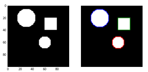
import numpy as npimport matplotlib.pyplot as pltfrom skimage import measure,draw #生成二值测试图像img=np.zeros([100,100])img[20:40,60:80]=1 #矩形rr,cc=draw.circle(60,60,10) #小圆rr1,cc1=draw.circle(20,30,15) #大圆img[rr,cc]=1img[rr1,cc1]=1#检测所有图形的轮廓contours = measure.find_contours(img, 0.5)#绘制轮廓fig, (ax0,ax1) = plt.subplots(1,2,figsize=(8,8))ax0.imshow(img,plt.cm.gray)ax1.imshow(img,plt.cm.gray)for n, contour in enumerate(contours): ax1.plot(contour[:, 1], contour[:, 0], linewidth=2)ax1.axis('image')ax1.set_xticks([])ax1.set_yticks([])plt.show()结果如下:不同的轮廓用不同的颜色显示
例2:
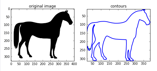
import matplotlib.pyplot as pltfrom skimage import measure,data,color#生成二值测试图像img=color.rgb2gray(data.horse())#检测所有图形的轮廓contours = measure.find_contours(img, 0.5)#绘制轮廓fig, axes = plt.subplots(1,2,figsize=(8,8))ax0, ax1= axes.ravel()ax0.imshow(img,plt.cm.gray)ax0.set_title('original image')rows,cols=img.shapeax1.axis([0,rows,cols,0])for n, contour in enumerate(contours): ax1.plot(contour[:, 1], contour[:, 0], linewidth=2)ax1.axis('image')ax1.set_title('contours')plt.show()
2、逼近多边形曲线
逼近多边形曲线有两个函数:subdivide_polygon()和 approximate_polygon()
subdivide_polygon()采用B样条(B-Splines)来细分多边形的曲线,该曲线通常在凸包线的内部。
函数格式为:
skimage.measure.subdivide_polygon(coords, degree=2, preserve_ends=False)
coords: 坐标点序列。
degree: B样条的度数,默认为2
preserve_ends: 如果曲线为非闭合曲线,是否保存开始和结束点坐标,默认为false
返回细分为的坐标点序列。
approximate_polygon()是基于Douglas-Peucker算法的一种近似曲线模拟。它根据指定的容忍值来近似一条多边形曲线链,该曲线也在凸包线的内部。
函数格式为:
skimage.measure.approximate_polygon(coords, tolerance)
coords: 坐标点序列
tolerance: 容忍值
返回近似的多边形曲线坐标序列。
例:
import numpy as npimport matplotlib.pyplot as pltfrom skimage import measure,data,color#生成二值测试图像hand = np.array([[1.64516129, 1.16145833], [1.64516129, 1.59375], [1.35080645, 1.921875], [1.375, 2.18229167], [1.68548387, 1.9375], [1.60887097, 2.55208333], [1.68548387, 2.69791667], [1.76209677, 2.56770833], [1.83064516, 1.97395833], [1.89516129, 2.75], [1.9516129, 2.84895833], [2.01209677, 2.76041667], [1.99193548, 1.99479167], [2.11290323, 2.63020833], [2.2016129, 2.734375], [2.25403226, 2.60416667], [2.14919355, 1.953125], [2.30645161, 2.36979167], [2.39112903, 2.36979167], [2.41532258, 2.1875], [2.1733871, 1.703125], [2.07782258, 1.16666667]])#检测所有图形的轮廓new_hand = hand.copy()for _ in range(5): new_hand =measure.subdivide_polygon(new_hand, degree=2)# approximate subdivided polygon with Douglas-Peucker algorithmappr_hand =measure.approximate_polygon(new_hand, tolerance=0.02)print("Number of coordinates:", len(hand), len(new_hand), len(appr_hand))fig, axes= plt.subplots(2,2, figsize=(9, 8))ax0,ax1,ax2,ax3=axes.ravel()ax0.plot(hand[:, 0], hand[:, 1],'r')ax0.set_title('original hand')ax1.plot(new_hand[:, 0], new_hand[:, 1],'g')ax1.set_title('subdivide_polygon')ax2.plot(appr_hand[:, 0], appr_hand[:, 1],'b')ax2.set_title('approximate_polygon')ax3.plot(hand[:, 0], hand[:, 1],'r')ax3.plot(new_hand[:, 0], new_hand[:, 1],'g')ax3.plot(appr_hand[:, 0], appr_hand[:, 1],'b')ax3.set_title('all')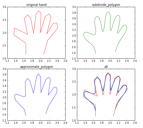
- python数字图像处理(17):边缘与轮廓
- python数字图像处理(17):边缘与轮廓
- python数字图像处理(17):边缘与轮廓
- 数字图像处理实验三 图像轮廓提取与边缘检测
- Python学习17_边缘与轮廓
- 【转】python-skimage的边缘与轮廓
- 数字图像处理 边缘检测
- (7)Air Band数字图像处理基础-边缘检测和轮廓跟踪
- 数字图像处理——轮廓
- 数字图像处理:8.边缘检测
- 数字图像处理之边缘检测
- 数字图像处理—图像分割—并行边界—利用边缘灰度不连续性(边缘)(边缘与导数)(边界闭合)
- 转载:数字图像处理——边缘检测算子(MATLAB)
- python数字图像处理(7):图像的形变与缩放
- python数字图像处理(8):对比度与亮度调整
- python数字图像处理(9):直方图与均衡化
- python数字图像处理(1):环境安装与配置
- python数字图像处理(7):图像的形变与缩放
- tar命令
- js实现图片预览和FormData上传
- Win7+OpenCV 2.4.13+Visual Studio 2015一劳永逸的配置
- android5.0以上获取系统进程信息
- 隐藏openssh 的版本号 (验证发现sshd服务重启报错,本篇暂时用作参考)
- python数字图像处理(17):边缘与轮廓
- js 数组随机排序
- 分类模型的评价
- 图形绘制: Canvas、SurfaceView、Paint、Surface、SurfaceHolder、Bitmap
- chmod命令简介
- hibernate之ID生成策略
- C# WPF MVVM 实战 – 5- 用绑定,通过 VM 设置 View 的控件焦点
- JAVA web 文件下载时 文件头设置
- 查找sqlserver查询死锁源头的方法 sqlserver死锁监控