TensorFlow框架(4)之CNN卷积神经网络详解
来源:互联网 发布:淘宝库存会影响排名吗 编辑:程序博客网 时间:2024/06/05 22:54
1. 卷积神经网络
1.1 多层前馈神经网络
多层前馈神经网络是指在多层的神经网络中,每层神经元与下一层神经元完全互连,神经元之间不存在同层连接,也不存在跨层连接的情况,如图 11所示。
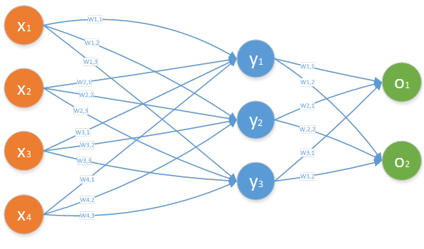
图 11
对于上图中隐藏层的第j个神经元的输出可以表示为:

其中,f是激活函数,bj为每个神经元的偏置。
1.2 卷积神经网络
1.2.1 网络结构
卷积神经网络与多层前馈神经网络的结构不一样,其每层神经元与下一层神经元不是全互连,而是部分连接,即每层神经层中只有部分的神经元与下一层神经元有连接,但是神经元之间不存在同层连接,也不存在跨层连接的情况,这两点与多层神经网络结构类似。如图 12所示。
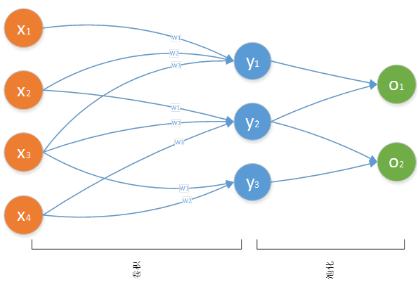
图 12
图 12中的输入层有4个神经元,但隐藏层的每个神经元只有3个输入,而图 11中的多层前馈神经网络结构中,隐藏层的每个神经元有4个输入层神经元的输入。
其中将输入层中的局部神经元称为局部感受野,如图 12所示中,(x1,x2,x3),(x2,x3,x4),(x3,x4)都为局部感受野。
1.2.2 卷积计算
卷积神经网络还有一点与前馈神经网络不同的,就是对于隐藏层中每个神经元共用一套输入权重,同时共享同一个偏置。所以对于图 12中隐藏层的第j个神经元的输出可以表示为:

i的区间是[0,1],f是激活函数,b为每个神经元的共享偏置。
其中将输入层到隐藏层中所共用的那一套权重和所共用那一个偏置,称为共享权重和共享偏置。
1.2.3 池化计算
从隐藏层到输出层也不是全连接结构,如图 12所示,也是隐藏层部分神经元连接到输出层神经元。同时隐藏层神经元到输出层神经元的计算方式有多种,如常用的最大值池化(max-pooling)法,输出层每个神经元选择从隐藏层连接到其神经元中最大的那个,如在图 12中y1,y2,y3的值分别为1,2,3。那么o1为2,o2为3.当然卷积神经网络的池化方法还有很多种,如L2法等。
1.2.4 特征映射
图 12中输入层只通过一套权重和一个偏置将输入层神经元映射到一个隐藏层,其实卷积神经网络可以通过多套权重和多个偏置将输入层映射为多个隐藏层。这些隐藏层是平行的。多少个特征映射完全取决于用户的计算需要。如图 13所示,第一次卷积运算时,一个输入层被映射为4个隐藏层(卷积层);第二次卷积运算时,每个输入层(池化层)被映射为3个隐藏层。所以经过第二次卷积后,总共有12个卷积层。
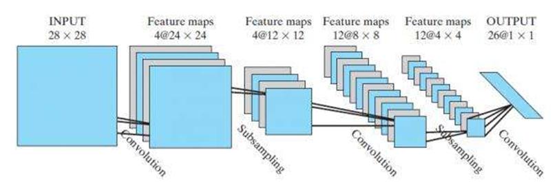
图 13
1.2.5 图像应用
上述介绍的卷积神经网络结构都是一维形式,即输入层、隐藏层和输出层都是一个向量形式。但是图像是一个二维结构,即一个矩阵形式。所以将卷积神经网络应用到图像识别上,需要转变一下思维,即将数据从一维转变到二维。
如图 14所示将一张28*28的图像(输入层)进行卷积运算,其中局部感受野为5*5。对于隐藏层的第一个像素点可以由输入层的前5*5矩形所有像素点进行计算而得,即

其中,i=0,j=0,若将式(3)转换为一维的,则可表示为:

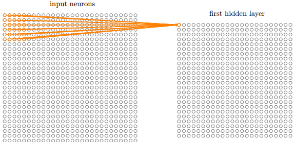
图 14
以此类推能计算出隐藏层的第二个像素点,如图 15所示,即通过公式可以表示为

其中,i=0,j=0,而且式(3)和式(5)中的权重wk,j和偏置b是相同的。
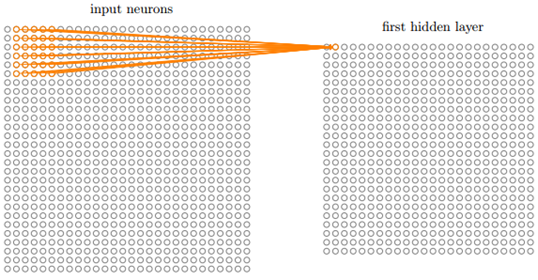
图 15
接着对隐藏层中的2*2矩形采用最大法进行池化,就能形成一个输出层,如图 16所示。
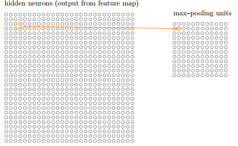
图 16
那么通过3组特征映射就能将一个输入层映射为3个隐藏层了,然后每个隐藏层能池化为一个输出层,如图 17所示的结构。
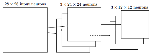
图 17
2. TensorFlow实现
2.1 API介绍
正如上述所介绍的,卷积神经网络有两个主要计算步骤:卷积和池化。TensorFlow为方便用户进行计算,提供了众多API来进行计算。
2.1.1 维度转换
由于在TensorFlow中常会出现输入数据维度与API接口行参维度不一致,如输入数据集为一个[784]结构的向量(数组),而API需要一个[28,28]结构的矩阵,那么就需要将一维(1-d)的向量转换为二维(2-d)的矩阵,当然保持数据不变。那么此时就可以使用TensorFlow提供的reshape函数。
def reshape(tensor, shape, name=None):
其中reshape函数的主要参数语义为:
- tensor:是需要被转换的tensor对象,可以是1-d、2-d或n-d结构;
- shape:指定了需要将tensor转换为什么结构的tensor,如上述可以传入为:[28,28].
# tensor 't' is [1, 2, 3, 4, 5, 6, 7, 8, 9]
# tensor 't' has shape [9]
reshape(t, [3, 3]) ==> [[1, 2, 3],
[4, 5, 6],
[7, 8, 9]]
# tensor 't' is [[[1, 1], [2, 2]],
# [[3, 3], [4, 4]]]
# tensor 't' has shape [2, 2, 2]
reshape(t, [2, 4]) ==> [[1, 1, 2, 2],
[3, 3, 4, 4]]
# tensor 't' is [[[1, 1, 1],
# [2, 2, 2]],
# [[3, 3, 3],
# [4, 4, 4]],
# [[5, 5, 5],
# [6, 6, 6]]]
# tensor 't' has shape [3, 2, 3]
# pass '[-1]' to flatten 't'
reshape(t, [-1]) ==> [1, 1, 1, 2, 2, 2, 3, 3, 3, 4, 4, 4, 5, 5, 5, 6, 6, 6]
# -1 can also be used to infer the shape
# -1 is inferred to be 9:
reshape(t, [2, -1]) ==> [[1, 1, 1, 2, 2, 2, 3, 3, 3],
[4, 4, 4, 5, 5, 5, 6, 6, 6]]
# -1 is inferred to be 2:
reshape(t, [-1, 9]) ==> [[1, 1, 1, 2, 2, 2, 3, 3, 3],
[4, 4, 4, 5, 5, 5, 6, 6, 6]]
# -1 is inferred to be 3:
reshape(t, [ 2, -1, 3]) ==> [[[1, 1, 1],
[2, 2, 2],
[3, 3, 3]],
[[4, 4, 4],
[5, 5, 5],
[6, 6, 6]]]
即若shape中某一维度指定的是-1,那么reshape会自动将数据填充到所指定的那一维中。
2.1.2 卷积操作
TensorFlow提供conv2d函数来实现神经网络的卷积运算,如下所示的定义:
def tf.nn.conv2d(input, filter, strides, padding, use_cudnn_on_gpu=None,
data_format=None, name=None)
主要参数语义为:
- batch:为待计算的批次数量,若是图像,则为图像的数量;
- in_height:为每张图像高度;
- in_width:为每张图像宽度;
- in_channels:为特征映射组的数量。
- filter_height:为局部感受野(或称核)的高度;
- filter_width:为局部感受野(或称核)的宽度;
- in_channels:为输入层的特征映射组的数量;
- out_channels:为输出层的特征映射组的数量;
如图 14的池化操作,可以按如下使用:
x_image = tf.reshape(x, [-1, 28, 28, 1])
initial_w = tf.truncated_normal([5, 5, 1, 3], stddev=0.1)
w=tf.Variable(initial_w)
initial_d = tf.constant(0.1, shape= [3])
d=tf.Variable(initial_d)
y=tf.nn.relu (tf.nn.conv2d(x_image, w )+d)
其中:
- x是一个2维(2-d)的图像输入,即是一个[none,784]的多张图像。为了适应conv2d图像的输入,所以将其转换为4维(4-d)的结构。由于指定的是share是[-1, 28, 28, 1],所以第一维是none数量值,而784会自动转换为28*28,最后一维都只有一个元素.
- 由于局部感受野是5*5,同时输入层中每张图像只有一组特征映射,同时生成的隐藏层中有3组特征映射,所以定义了结构是[5, 5, 1, 3]。
- 由于每个特征映射只有一个偏置,同时隐藏层中希望生成3组特征映射,所以偏置d为[3]结构。
- relu是TensorFlow提供的线性激活函数,其是一个[none,28,28,3]结构的tensor,因为不知道被计算图像的数量,所以是none;同时padding默认为'SAME',保持维度不变,所以仍未28*28.
2.1.3 池化操作
TensorFlow提供多个函数来实现神经网络的池化运算,由于池化函数定义的参数语义类似,所以这里只介绍其中的max_pool函数,如下是其定义:
def tf.nn. max_pool(value, ksize, strides, padding, data_format="NHWC", name=None):
主要参数语义为:
- batch:为待池化的数量,即图像的数量;
- height:每张图像的高度;
- width:每张图像的宽度;
- channels:为待池化图层中的特征映射组的数量。
- pool_height:为待池化层中矩形区域的高度;
- pool_width:为待池化层中矩形区域的宽度;
- strides_height:为向下移动的步长;
- strides_width:为向右移动的步长;
如所示的池化操作,可以用TensorFlow进行如下操作:
tf.nn.max_pool(y, ksize=[1, 2, 2, 1], strides=[1, 2, 2, 1], padding='SAME')
- y为上述经过池化后的数据,其是一个[none,28,28,3]结构的tensor;
- 由于隐藏层中每次以一个2*2的矩形进行池化,所以ksize为[1, 2, 2, 1];
- 池化操作不像卷积会出现像素点重叠,向右和向下以2个像素点移动,所以strides为[1, 2, 2, 1]。
2.2 多层卷积网络
2.2.1 辅助函数
为了后续计算方便,我们定义了如下四个函数:
def conv2d(x, W):
"""conv2d returns a 2d convolution layer with full stride."""
return tf.nn.conv2d(x, W, strides=[1, 1, 1, 1], padding='SAME')
def max_pool_2x2(x):
"""max_pool_2x2 downsamples a feature map by 2X."""
return tf.nn.max_pool(x, ksize=[1, 2, 2, 1],
strides=[1, 2, 2, 1], padding='SAME')
def weight_variable(shape):
"""weight_variable generates a weight variable of a given shape."""
initial = tf.truncated_normal(shape, stddev=0.1)
return tf.Variable(initial)
def bias_variable(shape):
"""bias_variable generates a bias variable of a given shape."""
initial = tf.constant(0.1, shape=shape)
return tf.Variable(initial)
2.2.2 第一次卷积和池化
获取的mnist数据,是以[6000,784]结构存在的tensor数据。为了能够使用TensorFlow的 tf.nn.conv2d 函数,所以需要将输入数据进行结构重置。
# grayscale -- it would be 3 for an RGB image, 4 for RGBA, etc.
x_image = tf.reshape(x, [-1, 28, 28, 1])
# First convolutional layer - maps one grayscale image to 32 feature maps.
W_conv1 = weight_variable([5, 5, 1, 32])
b_conv1 = bias_variable([32])
h_conv1 = tf.nn.relu(conv2d(x_image, W_conv1) + b_conv1)
# Pooling layer - downsamples by 2X.
h_pool1 = max_pool_2x2(h_conv1)
对于数据数据的每张图像是以[28,28]形式;通过卷积后,转变为[28,28,32]形式,其中32是其特征映射组的数量;再进行池化后,转变为[14,14,64]的形式。如图 21所示。
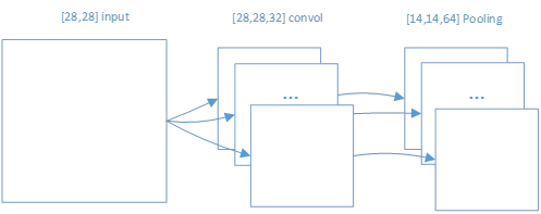
图 21
2.2.3 第二次卷积和池化
在第一次卷积和池化后生成的h_pool1对象是一个[None,14,14,64]的tensor。即对于第二次卷积来说,h_pool1就是一个输入tensor。如下所示的卷积和池化操作。
# Second convolutional layer -- maps 32 feature maps to 64.
W_conv2 = weight_variable([5, 5, 32, 64])
b_conv2 = bias_variable([64])
h_conv2 = tf.nn.relu(conv2d(h_pool1, W_conv2) + b_conv2)
# Second pooling layer.
h_pool2 = max_pool_2x2(h_conv2)
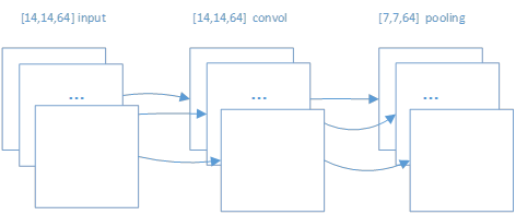
图 22
2.2.4 前馈神经网络
在两次卷积池化后,再采用传统前馈网络进行训练。第二次池化后的h_pool2对象是一个[None,7,7,64]的tensor,即一张图片从一开始输入,经过两次卷积池化后,变成一张有7*7*64个像素点的图像。
由于传统前馈网络的输入数据和输出数据是一个一维(1-d)结构,所以需要对h_pool2对象进行结构重置。
# Fully connected layer 1 -- after 2 round of downsampling, our 28x28 image
# is down to 7x7x64 feature maps -- maps this to 1024 features.
W_fc1 = weight_variable([7 * 7 * 64, 1024])
b_fc1 = bias_variable([1024])
h_pool2_flat = tf.reshape(h_pool2, [-1, 7*7*64])
h_fc1 = tf.nn.relu(tf.matmul(h_pool2_flat, W_fc1) + b_fc1)
如图 23所示的重置和全连接网络结构:
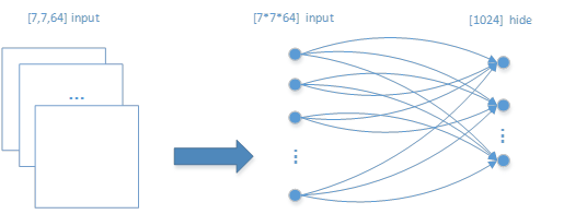
图 23
2.2.5 过拟合操作
# Dropout - controls the complexity of the model, prevents co-adaptation of
# features.
keep_prob = tf.placeholder(tf.float32)
h_fc1_drop = tf.nn.dropout(h_fc1, keep_prob)
2.2.6 生成输出标签
对于多层前馈神经网络有一个输入层和一个输出层,以及多个隐藏层。我们只实现一个隐藏层,所以这里直接将隐藏层转换为输出层,如下所示的程序:
# Map the 1024 features to 10 classes, one for each digit
W_fc2 = weight_variable([1024, 10])
b_fc2 = bias_variable([10])
y_conv = tf.matmul(h_fc1_drop, W_fc2) + b_fc2
结合图 23的输入层和隐藏层,增加了输出层,整个多层前馈神经网络的结构如图 24所示。
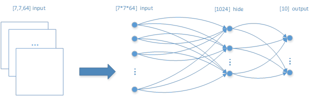
图 24
2.2.7 模型训练
每一张图像([784]类型的向量)通过多层前馈神经网络运算输出一个[10]向量后,此时可以使用softmax激活函数,生成一个[10]的标签,指明是哪一个阿拉伯数字了。如下所示进行数据训练的过程:
#创建优化器,使其来优化W和b等参数
cross_entropy = tf.reduce_mean(
tf.nn.softmax_cross_entropy_with_logits(labels=y_, logits=y_conv))
train_step = tf.train.AdamOptimizer(1e-4).minimize(cross_entropy)
#通过卷积和前馈网络计算后,有y_conv的预测值,所以能够将其与y_进行比较,从而测量其性能。
correct_prediction = tf.equal(tf.argmax(y_conv, 1), tf.argmax(y_, 1))
accuracy = tf.reduce_mean(tf.cast(correct_prediction, tf.float32))
with tf.Session() as sess:
sess.run(tf.global_variables_initializer())
for i in range(20000):
batch = mnist.train.next_batch(50)
if i % 100 == 0:
train_accuracy = accuracy.eval(feed_dict={
x: batch[0], y_: batch[1], keep_prob: 1.0})
print('step %d, training accuracy %g' % (i, train_accuracy))
train_step.run(feed_dict={x: batch[0], y_: batch[1], keep_prob: 0.5})
print('test accuracy %g' % accuracy.eval(feed_dict={
x: mnist.test.images, y_: mnist.test.labels, keep_prob: 1.0}))
3. 参考文献
4. 附录
该附录程序是来自 \tensorflow\examples\tutorials\mnist\mnist_deep.py。但是mnist数据存在本地的'/tmp/MNIST_data/'路径。
from __future__ import absolute_import
from __future__ import division
from __future__ import print_function
import argparse
import sys
from tensorflow.examples.tutorials.mnist import input_data
import tensorflow as tf
FLAGS = None
def deepnn(x):
"""deepnn builds the graph for a deep net for classifying digits.
Args:
x: an input tensor with the dimensions (N_examples, 784), where 784 is the
number of pixels in a standard MNIST image.
Returns:
A tuple (y, keep_prob). y is a tensor of shape (N_examples, 10), with values
equal to the logits of classifying the digit into one of 10 classes (the
digits 0-9). keep_prob is a scalar placeholder for the probability of
dropout.
"""
# Reshape to use within a convolutional neural net.
# Last dimension is for "features" - there is only one here, since images are
# grayscale -- it would be 3 for an RGB image, 4 for RGBA, etc.
x_image = tf.reshape(x, [-1, 28, 28, 1])
# First convolutional layer - maps one grayscale image to 32 feature maps.
W_conv1 = weight_variable([5, 5, 1, 32])
b_conv1 = bias_variable([32])
h_conv1 = tf.nn.relu(conv2d(x_image, W_conv1) + b_conv1)
# Pooling layer - downsamples by 2X.
h_pool1 = max_pool_2x2(h_conv1)
# Second convolutional layer -- maps 32 feature maps to 64.
W_conv2 = weight_variable([5, 5, 32, 64])
b_conv2 = bias_variable([64])
h_conv2 = tf.nn.relu(conv2d(h_pool1, W_conv2) + b_conv2)
# Second pooling layer.
h_pool2 = max_pool_2x2(h_conv2)
# Fully connected layer 1 -- after 2 round of downsampling, our 28x28 image
# is down to 7x7x64 feature maps -- maps this to 1024 features.
W_fc1 = weight_variable([7 * 7 * 64, 1024])
b_fc1 = bias_variable([1024])
h_pool2_flat = tf.reshape(h_pool2, [-1, 7*7*64])
h_fc1 = tf.nn.relu(tf.matmul(h_pool2_flat, W_fc1) + b_fc1)
# Dropout - controls the complexity of the model, prevents co-adaptation of
# features.
keep_prob = tf.placeholder(tf.float32)
h_fc1_drop = tf.nn.dropout(h_fc1, keep_prob)
# Map the 1024 features to 10 classes, one for each digit
W_fc2 = weight_variable([1024, 10])
b_fc2 = bias_variable([10])
y_conv = tf.matmul(h_fc1_drop, W_fc2) + b_fc2
return y_conv, keep_prob
def conv2d(x, W):
"""conv2d returns a 2d convolution layer with full stride."""
return tf.nn.conv2d(x, W, strides=[1, 1, 1, 1], padding='SAME')
def max_pool_2x2(x):
"""max_pool_2x2 downsamples a feature map by 2X."""
return tf.nn.max_pool(x, ksize=[1, 2, 2, 1],
strides=[1, 2, 2, 1], padding='SAME')
def weight_variable(shape):
"""weight_variable generates a weight variable of a given shape."""
initial = tf.truncated_normal(shape, stddev=0.1)
return tf.Variable(initial)
def bias_variable(shape):
"""bias_variable generates a bias variable of a given shape."""
initial = tf.constant(0.1, shape=shape)
return tf.Variable(initial)
def main(_):
# Import data
mnist = input_data.read_data_sets(FLAGS.data_dir, one_hot=True)
# Create the model
x = tf.placeholder(tf.float32, [None, 784])
# Define loss and optimizer
y_ = tf.placeholder(tf.float32, [None, 10])
# Build the graph for the deep net
y_conv, keep_prob = deepnn(x)
cross_entropy = tf.reduce_mean(
tf.nn.softmax_cross_entropy_with_logits(labels=y_, logits=y_conv))
train_step = tf.train.AdamOptimizer(1e-4).minimize(cross_entropy)
correct_prediction = tf.equal(tf.argmax(y_conv, 1), tf.argmax(y_, 1))
accuracy = tf.reduce_mean(tf.cast(correct_prediction, tf.float32))
with tf.Session() as sess:
sess.run(tf.global_variables_initializer())
for i in range(20000):
batch = mnist.train.next_batch(50)
if i % 100 == 0:
train_accuracy = accuracy.eval(feed_dict={
x: batch[0], y_: batch[1], keep_prob: 1.0})
print('step %d, training accuracy %g' % (i, train_accuracy))
train_step.run(feed_dict={x: batch[0], y_: batch[1], keep_prob: 0.5})
print('test accuracy %g' % accuracy.eval(feed_dict={
x: mnist.test.images, y_: mnist.test.labels, keep_prob: 1.0}))
if __name__ == '__main__':
parser = argparse.ArgumentParser()
parser.add_argument('--data_dir', type=str,
default='/tmp/MNIST_data/',
help='Directory for storing input data')
FLAGS, unparsed = parser.parse_known_args()
tf.app.run(main=main, argv=[sys.argv[0]] + unparsed)
- TensorFlow框架(4)之CNN卷积神经网络详解
- TensorFlow框架(4)之CNN卷积神经网络详解
- TensorFlow框架(4)之CNN卷积神经网络详解
- tensorflow CNN卷积神经网络
- tensorflow CNN卷积神经网络
- TensorFlow实现卷积神经网络CNN
- TensorFlow学习--卷积神经网络CNN
- TensorFlow搭建CNN卷积神经网络
- TensorFlow实现卷积神经网络CNN
- TensorFlow -- 实现CNN卷积神经网络
- 详解卷积神经网络(CNN)
- 详解卷积神经网络(CNN)
- Tensorflow深度学习之二:简单卷积神经网络CNN
- tensorflow之简单卷积神经网络(CNN)搭建
- Tensorflow之 CNN卷积神经网络的MNIST手写数字识别
- 【TensorFlow】TensorFlow 的卷积神经网络 CNN
- Deep Learning-TensorFlow (7) CNN卷积神经网络_《Tensorflow:实战Google深度学习框架》
- 卷积神经网络CNN原理以及TensorFlow实现
- SSH(进阶) SpringDataJPA + SpringMVC 快速搭建企业框架
- centos安装vmvaretools
- 将oracle数据库的数据导入mysql
- 【C#】Attribute
- 平衡二叉树的判断
- TensorFlow框架(4)之CNN卷积神经网络详解
- 2015年终总结
- 安装机器人ros驱动遇到的问题(catkin_make)
- 用string剖析浅拷贝、深拷贝、写时拷贝
- delphi字符串切割
- javascript实现字典数据结构
- activity中 调用startActivityForResult的步骤及生命周期
- codeforces 849B Tell Your World
- python中判断一个数字是否是质数