Andrew NG机器学习线性回归编程作业

备注: Coursera上Andrew Ng的机器学习课程有8次编程作业。本帖记录我练习过程中学到的知识，希望对大家有帮助。Andrew NG机器学习线性回归编程作业详细分析，这篇耗费巨大心血，非常适合小白去做NG课程作业时参考，部分代码不好理解（先放弃），重点理解NG留的那些空的代码，然后参考我整理的另一篇博客，线性规划的Matlab代码总结，结合着看，慢慢就懂了，加油

---

背景

在本次练习中，需要实现一个单变量的线性回归。假设有一组历史数据<城市人口，开店利润>，现需要预测在哪个城市中开店利润比较好？

历史数据如下：第一列表示城市人口数，单位为万人；第二列表示利润，单位为10,000$

    5.5277    9.1302    8.5186   13.6620    7.0032   11.8540    .....    ......

---

补充matlab知识

1. Matlab的工作目录
   使用matlab中图形化的Current Folder面板可以修改当前工作目录
   
   只有进入工作目录， Matlab才能默认找到该目录下的各种文件。

2. 可以使用命令来调整工作目录
   pwd 查看当前工作目录
   用于当前工作目录的路径。例如：

   pwd
   ans =C:\MATLAB7\work

   cd 进入某目录，用于切换当前工作目录。例如：

   cd(‘c:/toolbox/matlab/demos’) %切换当前工作目录到demos
   cd .. %切换当前工作目录到matlab

   ls 列出当前目录下的内容
   直接打出ls就可以

3. m脚本文件
   matlab是解释型的语言，在命令行界面可以输入命令执行。脚本文件就是把多个命令合在一起，在命令行调用这个脚本文件就可以执行文件里面的一句句命令。
   例如在命令行输入两条命令
   
   执行后可以在Workspace窗口看到已有的变量
   
   我们也可以使用脚本文件来完成相同的事情。新建一个文件，内容为
   c = 7
d = c*7

   保存到当前工作目录下，命名script1.m。然后在命令界面输入script1，就相当于执行了文件里的这两条语句。之后在Workspace窗口可以看到变量c和d。
   备注：matlab 的editor怎么打开？
   直接点File下的新建m文件图标
   Ctrl+N

4. m函数文件
   函数文件用来定义matlab中的函数，可以供上层调用。 函数文件要保存为 函数名.m ，才可以通过函数名来调用。经过我的测试，文件名和文件中的函数名不一致时，以文件名为准。

function 返回值 = 函数名(输入参数)           % YOUR CODE HERE End

返回值和输入参数都可以有多个，之间用逗号隔开。返回值有多个的时候要用方括号包起来。

function [返回值1, 返回值2] = 函数名(输入1，输入2，输入3)             % YOUR CODE HERE End

示例：
我们新建一个f1.m，内容如下

function s = f1(a) s = a+8; end

保存到工作目录后就可以使用这个函数

5.语句中的分号
语句不带分号会输出运行结果，如果语句带分号则不输出结果。

6.第一次编程作业的文件如下图

脚本文件ex1用来执行单变量线性回归，ex1_multi.m用来执行多变量线性回归。submit.m用来提交你的作业到服务器，本文不包含对这部分代码的分析。

编程过程及其理解

1.初始化Initialization

%% Initializationclear all; close all; clc

备注：
1.两个百分号%%是matlab中用来表示代码块的注释。从%%开始到下一个%%之间会作为一个代码块，在matlab中查看时会用黄白相间显示
2.clear 清除工作区的所有变量。还可以后面跟变量名来清除某个变量。
3.close all 关闭所有窗口（显示图像的figure窗口）
4.clc 清除命令窗口的内容（就是命令界面以前的命令）
5.% 代表注释行

2. 基础函数 Part 1:Basic Function

% Complete warmUpExercise.m fprintf('Running warmUpExercise ... \n');fprintf('5x5 Identity Matrix: \n');warmUpExercise()fprintf('Program paused. Press enter to continue.\n');pause;

完成warmUpExercise.m 的函数
注释：
1.fprintf的用法
fprintf和c语言中的printf用法类似，用于格式化输出，也支持%d等占位符，也可以直接输出字符串，\n表示换行符。Matlab中字符串用单引号括起来。fprintf函数可以将数据按指定格式写入到文本文件中。
数据的格式化输出：fprintf(fid,format,variables)
按指定的格式将变量的值输出到屏幕或指定文件
fid为文件句柄，若缺省，则输出到屏幕
format用来指定数据输出时采用的格式
%d 整数
%e实数：科学计算法形式
%f实数：小数形式
%g由系统自动选取上述两种格式之一
%s输出字符串
fprintf(fid，format，A)
说明：fid为文件句柄，指定要写入数据的文件，format是用来控制所写数据格式的格式符，与fscanf函数相同，A是用来存放数据的矩阵。
2.\n是换行，英文是New line，表示使光标到行首。
\r是回车，英文是Carriage return，表示使光标下移一格。
3.pause用来暂停。
中间调用了warmUpExercise函数，也就是warmUpExercise.m对应的函数。这个函数要求输出一个5*5的单位矩阵，直接使用eye函数就可以了。
3.函数warmUpExercise()如下

function A = warmUpExercise()A = [];A = eye(5);end

注释：
1.A= [ ] ，A是空矩阵
2.eye() ，单位矩阵

输入参数无，返回值A。
之后在命令界面可以调用这个函数

4. 画图Part 2: Plotting

fprintf('Plotting Data ...\n')data = csvread('ex1data1.txt');X = data(:, 1); y = data(:, 2);m = length(y);plotData(X, y);fprintf('Program paused. Press enter to continue.\n');pause;

注释：
1.data = csvread(‘ex1data1.txt’)和data = load(‘ex1data1.txt’);意思一样都是加载数据，使用load函数来读取文件，会自动返回生成的矩阵
2.CSVREAD（）函数用法
第一种：M = CSVREAD(‘FILENAME’) ，直接读取csv文件的数据，并返回给M
第二种：M = CSVREAD(‘FILENAME’,R,C) ，读取csv文件中从第R-1行，第C-1列的数据开始的数据，这对带有头文件说明的csv文件(如示波器等采集的文件)的读取是很重要的。
第三种：M = CSVREAD(‘FILENAME’,R,C,RNG)，其中 RNG = [R1 C1 R2 C2]，读取左上角为索引为(R1,C1) ,右下角索引为(R2,C2)的矩阵中的数据。
P.S：matlab认为CSV第1行第1列的单元格坐标为（0,0）
csvread函数只试用与用逗号分隔的纯数字文件

3.该部分先从文件读取数据，然后调用plotData来画图，在工作区窗口可以看到data的类型97行2列的矩阵。可以看出ex1data1.txt中有97行数据。

4.

• Matlab中矩阵和向量的下标都是从1开始 ，而不像c语言中从0开始。
  下面的代码把data矩阵的第一列给X，第2列给y。X和y的类型都是列向量（n*1矩阵）。
  X = data(:, 1); y = data(:, 2);
• 引用矩阵中的元素是通过括号。假设a是一个m*n矩阵
  a(3,4)就是a的第3行第4列的元素。

5.冒号表示所有
a(:,4)表示矩阵a的第4列元素，这个结果是列向量（m*1矩阵）
a(3,:)表示a的第3行元素，是行向量（1*n矩阵）
引用向量中的元素时，括号里只有1个数字，例如b是向量
b(3)表示b中第3个元素。

6.m = length(y); length函数，返回向量y的长度。这也是我们的训练集中实例的个数。
7.最后调用plotData(X, y)来画图。

5.函数plotData（）如下

 function plotData(x, y) figure; % open a new figure window plot(x, y, 'rx', 'MarkerSize', 10); % Plot the data ylabel('Profit in $10,000s'); % Set the yaxis label xlabel('Population of City in 10,000s'); % Set the xaxis label End

注释：
1. figure; 表示打开一个新的画图窗口
2. plot用来画点。’rx’表示红色，x型。’MarkerSize’, 10 表示大小是10 。plot的用法非常灵活，可以参考 官方文档 。此处的格式为
plot(X1,Y1,LineSpec, ‘PropertyName’, PropertyValue,…)

3.xlabel和ylabel用于设置坐标说明。
在我们的脚本ex1中，X存放了数据第一列，y存放了数据的第二列，调用画图函数就可以画出散点图了

6.梯度下降Part 3: Gradient descent

%% ======== Part 3: Gradient descent ===================fprintf('Running Gradient Descent ...\n')X = [ones(m, 1), data(:,1)]; % Add a column of ones to xtheta = zeros(2, 1); % initialize fitting parameters% Some gradient descent settingsiterations = 1500;alpha = 0.01;% compute and display initial costcomputeCost(X, y, theta)% run gradient descenttheta = gradientDescent(X, y, theta, alpha, iterations);% print theta to screenfprintf('Theta found by gradient descent: ');fprintf('%f %f \n', theta(1), theta(2));% Plot the linear fithold on; % keep previous plot visibleplot(X(:,2), X*theta, '-')legend('Training data', 'Linear regression')hold off % don't overlay any more plots on this figure% Predict values for population sizes of 35,000 and 70,000predict1 = [1, 3.5] *theta;fprintf('For population = 35,000, we predict a profit of %f\n',...    predict1*10000);predict2 = [1, 7] * theta;fprintf('For population = 70,000, we predict a profit of %f\n',...    predict2*10000);fprintf('Program paused. Press enter to continue.\n');pause;

注释：
1.
ones（x,y） X行Y列的单位阵
zeros(x,y) X行Y 列的零矩阵
2.hold on 和hold off是相对使用的：
前者的意思是，你在当前图的轴（坐标系）中画了一幅图，再画另一幅图时，原来的图还在，与新图共存，都看得到；
后者表达的是，你在当前图的轴（坐标系）中画了一幅图，此时，状态是hold off,则再画另一幅图时，原来的图就看不到了，在轴上绘制的是新图，原图被替换了。
3.第4行 X = [ones(m, 1), data(:,1)] ，是给X最左边添加一列，全为1
4.
C语言中’\n’是换行的意思，一般放到printf()这类函数中使用，比如：
printf(“this is a test\n Please check it\n”);
结果是：
this is a test
Please check it
5.computeCost(X, y, theta)函数用来计算代价
6.theta = zeros(2, 1)，设置参数theta的初值，此处设置的初值都是0
7.假设函数、代价函数和梯度下降算法的向量表示
假设函数的向量表示如下：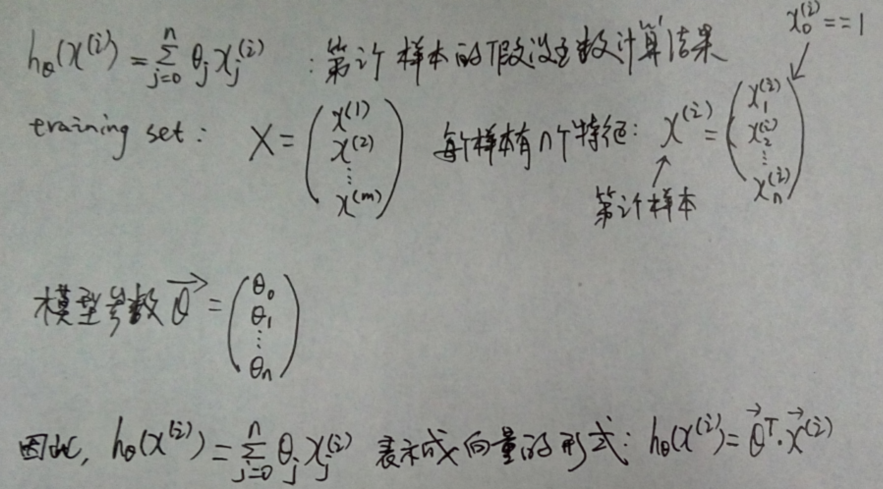

代价函数的表示如下：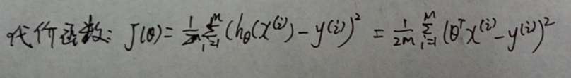

使用梯度下降算法求解 θ 的向量表示如下：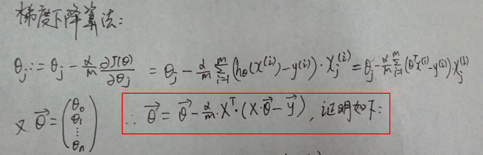

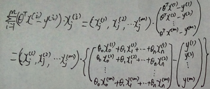
证明过程如下：

8.matlab的legend用法
用Matlab画图时，有时候需要对各种图标进行标注，例如，用“+”代表A的运动情况，“*”代表B的运动情况。

legend函数的基本用法是：

LEGEND(string1,string2,string3, …)

分别将字符串1、字符串2、字符串3……标注到图中，每个字符串对应的图标为画图时的图标。
例如:

plot(x,sin(x),’.b’,x,cos(x),’+r’)

legend(‘sin’,’cos’)这样可以把”.”标识为’sin’，把”+”标识为”cos”

还可以用LEGEND(…,’Location’,LOC) 来指定图例标识框的位置。
7.computeCost()函数

function J = computeCost(X, y, theta)m = length(y);J = 0;J = sum((X*theta - y).^2) / (2 * m);end

注释：
1.此时

2.函数sum( )的用法
a=sum(x); %列求和
a=sum(x,2)； %行求和
a=sum(x(:)); %矩阵求和
假定x为一个矩阵：
sum(x)以矩阵x的每一列为对象，对一列内的数字求和。
sum(x,2)以矩阵x的每一行为对象，对一行内的数字求和。

3.
这个求和可以用循环来解决，不过matlab的专长是矩阵，我们应该利用向量和矩阵的特点实现同时计算多个变量。这叫做向量化计算，是非常重要的。
这里说一下matlab中的运算符，基本的有四则运算+ – * /和^幂运算,如果是两个矩阵运算，会按照矩阵运算的规则，
例如矩阵乘法和矩阵除法（乘以逆矩阵）。如果想对矩阵中的每个元素做计算，要使用点号. ，例如矩阵A和矩阵B对应位置元素相乘，应该用 A .* B另外，矩阵和标量做运算，结果是对矩阵中每个元素做运算。例如A中每个月元素加2，A+2

先来看求和号里面的第i项，对应第i个数据。
先用一个变量求出h(x)
hx = X * theta
注意个矩阵运算的结果中包含了i从0到m所有的结果

此时X是一个m*2的矩阵，theta是一个2*1的矩阵

这里用 .^ 表示对矩阵中每个元素平方，而不是求矩阵的平方。
上面的向量所有元素加起来就是累加结果
sum((hx – y).^2)
最后求得J
J = sum((hx – y).^2) / (2*m)
备注：function [输出变量] = 函数名称(输入变量）
8. 梯度下降函数gradientDescent(）

function [theta, J_history] = gradientDescent(X, y, theta, alpha, num_iters)              %定义梯度下降函数m = length(y);          %训练实例的个数for iter = 1:num_iters        H = X * theta;%假设函数        T = [0 ; 0];%     for i = 1 : m,        T = T + (H(i) - y(i)) * X(i,:)';     end    theta = theta - (alpha * T) / m;     J_history(iter) = computeCost(X, y, theta);endend

注释：
1.J_history用来记录每次迭代时的代价值。
2.先表示求和号里面，第j个参数对应的是
3. X(i,:)’表示第i行所有元素进行转置
4. 用手抄代码整理出来。会贴在此处。

9.Part 4: Visualizing J(theta_0, theta_1)

%% ====== Part 4: Visualizing J(theta_0, theta_1) =============fprintf('Visualizing J(theta_0, theta_1) ...\n')% Grid over which we will calculate Jtheta0_vals = linspace(-10, 10, 100);theta1_vals = linspace(-1, 4, 100);% initialize J_vals to a matrix of 0'sJ_vals = zeros(length(theta0_vals), length(theta1_vals));% Fill out J_valsfor i = 1:length(theta0_vals)    for j = 1:length(theta1_vals)      t = [theta0_vals(i); theta1_vals(j)];          J_vals(i,j) = computeCost(X, y, t);    endend% Because of the way meshgrids work in the surf command, we need to % transpose J_vals before calling surf, or else the axes will be flippedJ_vals = J_vals';% Surface plotfigure;surf(theta0_vals, theta1_vals, J_vals)xlabel('\theta_0'); ylabel('\theta_1');% Contour plotfigure;% Plot J_vals as 15 contours spaced logarithmically between 0.01 and 100contour(theta0_vals, theta1_vals, J_vals, logspace(-2, 3, 20))xlabel('\theta_0'); ylabel('\theta_1');hold on;plot(theta(1), theta(2), 'rx', 'MarkerSize', 10, 'LineWidth', 2);

注释：
1.linspace的用法
2.具体画图这个不具体分析，目前功力不够

？？？？？？？？？？？看不懂

10. 多变量代价函数computeCostMulti（）

function J = computeCostMulti(X, y, theta)m = length(y); % number of training examplesJ = 0;% ====================== YOUR CODE HERE ======================J = sum((X * theta - y).^2) / (2 * m);% ==========================================================end

11.多变量的梯度下降函数 gradientDescentMulti（）

function [theta, J_history] = gradientDescentMulti(X, y, theta, alpha, num_iters)%GRADIENTDESCENTMULTI Performs gradient descent to learn theta%   theta = GRADIENTDESCENTMULTI(x, y, theta, alpha, num_iters) updates theta by%   taking num_iters gradient steps with learning rate alpha% Initialize some useful valuesm = length(y); % number of training examplesn = size(X , 2);J_history = zeros(num_iters, 1);for iter = 1:num_iters    % ====================== YOUR CODE HERE ======================    % Instructions: Perform a single gradient step on the parameter vector    %               theta.     %    % Hint: While debugging, it can be useful to print out the values    %       of the cost function (computeCostMulti) and gradient here.    %    H = X * theta;    T = zeros(n , 1);    for i = 1 : m,        T = T + (H(i) - y(i)) * X(i,:)';        end    theta = theta - (alpha * T) / m;    % ============================================================    % Save the cost J in every iteration        J_history(iter) = computeCostMulti(X, y, theta);endend

**注释：
由于单变量中我们的计算方法同样适用于多变量，这里的代码不需要改变，直接用ex1中的代码即可。**
12.特征归一化Feature Normalization

%% ======= Part 1: Feature Normalization ================%% Clear and Close Figuresclear all; close all; clcfprintf('Loading data ...\n');%% Load Datadata = csvread('ex1data2.txt');X = data(:, 1:2);y = data(:, 3);m = length(y);% Print out some data pointsfprintf('First 10 examples from the dataset: \n');fprintf(' x = [%.0f %.0f], y = %.0f \n', [X(1:10,:) y(1:10,:)]');fprintf('Program paused. Press enter to continue.\n');pause;% Scale features and set them to zero meanfprintf('Normalizing Features ...\n');[X mu sigma] = featureNormalize(X);% Add intercept term to XX = [ones(m, 1) X];

13.特征归一化函数featureNormalize(X)

function [X_norm, mu, sigma] = featureNormalize(X)%FEATURENORMALIZE Normalizes the features in X %   FEATURENORMALIZE(X) returns a normalized version of X where%   the mean value of each feature is 0 and the standard deviation%   is 1. This is often a good preprocessing step to do when%   working with learning algorithms.% You need to set these values correctlyX_norm = X;mu = zeros(1, size(X, 2));sigma = zeros(1, size(X, 2));% ====================== YOUR CODE HERE ======================% Instructions: First, for each feature dimension, compute the mean%               of the feature and subtract it from the dataset,%               storing the mean value in mu. Next, compute the %               standard deviation of each feature and divide%               each feature by it's standard deviation, storing%               the standard deviation in sigma. %%               Note that X is a matrix where each column is a %               feature and each row is an example. You need %               to perform the normalization separately for %               each feature. %% Hint: You might find the 'mean' and 'std' functions useful.%       m = size(X , 1);mu = mean(X);for i = 1 : m,    X_norm(i, :) = X(i , :) - mu;endsigma = std(X);for i = 1 : m,    X_norm(i, :) = X_norm(i, :) ./ sigma;end%mu , sigma , X_norm% ============================================================end

注释：
由于缩放之后，输入新参数预测的时候，需要对输入做相同的缩放，才可以得出正确的结果，因此此函数返回了缩放时用到的均值和标准差。
使用到了mean和std函数，可以在matlab中使用help mean和help std来查看用法。
可以求出每列的均值和标准差，之后可以对每行进行缩放
mu = mean(X);
sigma = std(X);
for i=1:size(X,1)
X_norm(i, :) = (X(i, :) - mu) ./ sigma;
End
也可以采用空间换时间的方法，把mu和sigma拷贝一份复制成多行的 就可以直接用元素对应运算了

13.梯度下降Gradient Descent

%% ======== Part 2: Gradient Descent ================% ====================== YOUR CODE HERE ======================fprintf('Running gradient descent ...\n');alpha = 0.3;num_iters = 100;theta = zeros(3, 1);[theta, J_history] = gradientDescentMulti(X, y, theta, alpha, num_iters);figure;plot(1:numel(J_history), J_history, '-b', 'LineWidth', 2);xlabel('Number of iterations');ylabel('Cost J');fprintf('Theta computed from gradient descent: \n');fprintf(' %f \n', theta);fprintf('\n');============================================================fprintf(['Predicted price of a 1650 sq-ft, 3 br house ' ...         '(using gradient descent):\n $%f\n'], price);fprintf('Program paused. Press enter to continue.\n');pause;

注释：
ex1_multi.m的第85行可以修改学习率。经过试验，学习率和迭代步数适当增加后，可以得到和正规方程相同的结果
14.正规方程 Normal Equations

%% ================ Part 3: Normal Equations ================fprintf('Solving with normal equations...\n');% ====================== YOUR CODE HERE ======================% Instructions: The following code computes the closed form %               solution for linear regression using the normal%               equations. You should complete the code in %               normalEqn.m%%               After doing so, you should complete this code %               to predict the price of a 1650 sq-ft, 3 br house.%%% Load Datadata = csvread('ex1data2.txt');X = data(:, 1:2);y = data(:, 3);m = length(y);% Add intercept term to XX = [ones(m, 1) X];% Calculate the parameters from the normal equationtheta = normalEqn(X, y);% Display normal equation's resultfprintf('Theta computed from the normal equations: \n');fprintf(' %f \n', theta);fprintf('\n');% Estimate the price of a 1650 sq-ft, 3 br house% ====================== YOUR CODE HERE ======================price = 0; % You should change this% ============================================================fprintf(['Predicted price of a 1650 sq-ft, 3 br house ' ...         '(using normal equations):\n $%f\n'], price);

关键代码
computeCost

J=sum((X*theta-y).^2)/(2*m);

gradientDescent

theta = theta - (1/m)*alpha*(X.'*(X*theta-y));J_history(iter) = computeCost(X, y, theta);

featureNormalize

mu=mean(X,1);sigma = std(X);X_norm = (X - ones(size(X, 1), 1) * mu) ./ (ones(size(X, 1), 1) * sigma);

computeCostMulti

J = (X * theta - y).' * (X * theta - y) / (2*m);

gradeDescentMulti

theta = theta - (1/m)*alpha*(X.'*(X*theta-y));J_history(iter) = computeCostMulti(X, y, theta);

normalEqn

theta=(inv(X.'*X))*X.'*y;