Regularization for DNN

Regularization

There are several ways of controlling the capacity of Neural Networks to prevent overfitting:

L2 regularization is perhaps the most common form of regularization. It can be implemented by penalizing the squared magnitude of all parameters directly in the objective. That is, for every weight ww in the network, we add the term 12λw212λw2 to the objective, where λλ is the regularization strength. It is common to see the factor of 1212 in front because then the gradient of this term with respect to the parameter ww is simply λwλw instead of 2λw2λw. The L2 regularization has the intuitive interpretation of heavily penalizing peaky weight vectors and preferring diffuse weight vectors. As we discussed in the Linear Classification section, due to multiplicative interactions between weights and inputs this has the appealing property of encouraging the network to use all of its inputs a little rather that some of its inputs a lot. Lastly, notice that during gradient descent parameter update, using the L2 regularization ultimately means that every weight is decayed linearly: W += -lambda * W towards zero.

L1 regularization is another relatively common form of regularization, where for each weight ww we add the term λ∣w∣λ∣w∣ to the objective. It is possible to combine the L1 regularization with the L2 regularization: λ1∣w∣+λ2w2λ1∣w∣+λ2w2(this is called Elastic net regularization). The L1 regularization has the intriguing property that it leads the weight vectors to become sparse during optimization (i.e. very close to exactly zero). In other words, neurons with L1 regularization end up using only a sparse subset of their most important inputs and become nearly invariant to the “noisy” inputs. In comparison, final weight vectors from L2 regularization are usually diffuse, small numbers. In practice, if you are not concerned with explicit feature selection, L2 regularization can be expected to give superior performance over L1.

Max norm constraints. Another form of regularization is to enforce an absolute upper bound on the magnitude of the weight vector for every neuron and use projected gradient descent to enforce the constraint. In practice, this corresponds to performing the parameter update as normal, and then enforcing the constraint by clamping the weight vector w⃗ w→ of every neuron to satisfy ∥w⃗ ∥2<c‖w→‖2<c. Typical values of cc are on orders of 3 or 4. Some people report improvements when using this form of regularization. One of its appealing properties is that network cannot “explode” even when the learning rates are set too high because the updates are always bounded.

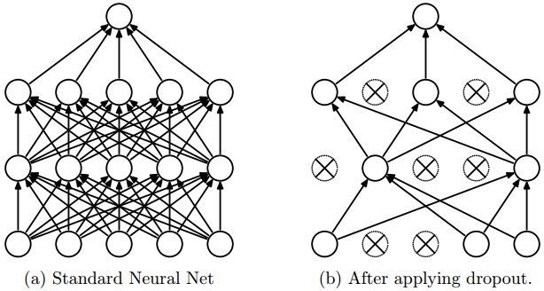
Dropout is an extremely effective, simple and recently introduced regularization technique by Srivastava et al. in Dropout: A Simple Way to Prevent Neural Networks from Overfitting (pdf) that complements the other methods (L1, L2, maxnorm). While training, dropout is implemented by only keeping a neuron active with some probability pp (a hyperparameter), or setting it to zero otherwise.

Figure taken from the Dropout paper that illustrates the idea. During training, Dropout can be interpreted as sampling a Neural Network within the full Neural Network, and only updating the parameters of the sampled network based on the input data. (However, the exponential number of possible sampled networks are not independent because they share the parameters.) During testing there is no dropout applied, with the interpretation of evaluating an averaged prediction across the exponentially-sized ensemble of all sub-networks (more about ensembles in the next section).

Vanilla dropout in an example 3-layer Neural Network would be implemented as follows:

""" Vanilla Dropout: Not recommended implementation (see notes below) """p = 0.5 # probability of keeping a unit active. higher = less dropoutdef train_step(X):  """ X contains the data """    # forward pass for example 3-layer neural network  H1 = np.maximum(0, np.dot(W1, X) + b1)  U1 = np.random.rand(*H1.shape) < p # first dropout mask  H1 *= U1 # drop!  H2 = np.maximum(0, np.dot(W2, H1) + b2)  U2 = np.random.rand(*H2.shape) < p # second dropout mask  H2 *= U2 # drop!  out = np.dot(W3, H2) + b3    # backward pass: compute gradients... (not shown)  # perform parameter update... (not shown)  def predict(X):  # ensembled forward pass  H1 = np.maximum(0, np.dot(W1, X) + b1) * p # NOTE: scale the activations  H2 = np.maximum(0, np.dot(W2, H1) + b2) * p # NOTE: scale the activations  out = np.dot(W3, H2) + b3

In the code above, inside the train_step function we have performed dropout twice: on the first hidden layer and on the second hidden layer. It is also possible to perform dropout right on the input layer, in which case we would also create a binary mask for the input X. The backward pass remains unchanged, but of course has to take into account the generated masks U1,U2.

Crucially, note that in the predict function we are not dropping anymore, but we are performing a scaling of both hidden layer outputs by pp. This is important because at test time all neurons see all their inputs, so we want the outputs of neurons at test time to be identical to their expected outputs at training time. For example, in case of p=0.5p=0.5, the neurons must halve their outputs at test time to have the same output as they had during training time (in expectation). To see this, consider an output of a neuron xx (before dropout). With dropout, the expected output from this neuron will become px+(1−p)0px+(1−p)0, because the neuron’s output will be set to zero with probability 1−p1−p. At test time, when we keep the neuron always active, we must adjust x→pxx→px to keep the same expected output. It can also be shown that performing this attenuation at test time can be related to the process of iterating over all the possible binary masks (and therefore all the exponentially many sub-networks) and computing their ensemble prediction.

The undesirable property of the scheme presented above is that we must scale the activations by pp at test time. Since test-time performance is so critical, it is always preferable to use inverted dropout, which performs the scaling at train time, leaving the forward pass at test time untouched. Additionally, this has the appealing property that the prediction code can remain untouched when you decide to tweak where you apply dropout, or if at all. Inverted dropout looks as follows:

""" Inverted Dropout: Recommended implementation example.We drop and scale at train time and don't do anything at test time."""p = 0.5 # probability of keeping a unit active. higher = less dropoutdef train_step(X):  # forward pass for example 3-layer neural network  H1 = np.maximum(0, np.dot(W1, X) + b1)  U1 = (np.random.rand(*H1.shape) < p) / p # first dropout mask. Notice /p!  H1 *= U1 # drop!  H2 = np.maximum(0, np.dot(W2, H1) + b2)  U2 = (np.random.rand(*H2.shape) < p) / p # second dropout mask. Notice /p!  H2 *= U2 # drop!  out = np.dot(W3, H2) + b3    # backward pass: compute gradients... (not shown)  # perform parameter update... (not shown)  def predict(X):  # ensembled forward pass  H1 = np.maximum(0, np.dot(W1, X) + b1) # no scaling necessary  H2 = np.maximum(0, np.dot(W2, H1) + b2)  out = np.dot(W3, H2) + b3

There has a been a large amount of research after the first introduction of dropout that tries to understand the source of its power in practice, and its relation to the other regularization techniques. Recommended further reading for an interested reader includes:

• Dropout paper by Srivastava et al. 2014.
• Dropout Training as Adaptive Regularization: “we show that the dropout regularizer is first-order equivalent to an L2 regularizer applied after scaling the features by an estimate of the inverse diagonal Fisher information matrix”.

Theme of noise in forward pass. Dropout falls into a more general category of methods that introduce stochastic behavior in the forward pass of the network. During testing, the noise is marginalized over analytically (as is the case with dropout when multiplying by pp), or numerically (e.g. via sampling, by performing several forward passes with different random decisions and then averaging over them). An example of other research in this direction includes DropConnect, where a random set of weights is instead set to zero during forward pass. As foreshadowing, Convolutional Neural Networks also take advantage of this theme with methods such as stochastic pooling, fractional pooling, and data augmentation. We will go into details of these methods later.

Bias regularization. As we already mentioned in the Linear Classification section, it is not common to regularize the bias parameters because they do not interact with the data through multiplicative interactions, and therefore do not have the interpretation of controlling the influence of a data dimension on the final objective. However, in practical applications (and with proper data preprocessing) regularizing the bias rarely leads to significantly worse performance. This is likely because there are very few bias terms compared to all the weights, so the classifier can “afford to” use the biases if it needs them to obtain a better data loss.

Per-layer regularization. It is not very common to regularize different layers to different amounts (except perhaps the output layer). Relatively few results regarding this idea have been published in the literature.

In practice: It is most common to use a single, global L2 regularization strength that is cross-validated. It is also common to combine this with dropout applied after all layers. The value of p=0.5p=0.5 is a reasonable default, but this can be tuned on validation data.