【译文】构建一个图书推荐系统 – 基础知识、knn算法和矩阵分解

作者 Susan Li

译者 钱亦欣

几乎每个人都有过过在某些网站被个性化推销商品的经历，亚马逊会告诉你购买这本书的读者还购买了…，Udemy则会显示浏览了这些课程的学生也浏览了…。Netfilix于2009年拿出了100万刀的奖金，举办了一个以将公司推荐精确度提高10个百分点为目标的数据大赛。

闲言少叙，如果你想从头学习如何架构一个推荐系统，就接着往下读。

数据

Book-Crossings 是一个由 Cai-Nicolas Ziegler 整理的关于图书评分的数据集。它有由90000位读者对270000本书籍做出了1100000万条评分记录，评分数据再1到10之间。

这个数据集共有三张表：评分表，书籍基本信息表和读者表，可以从此处下载。

import pandas as pdimport numpy as npimport matplotlib.pyplot as pltbooks = pd.read_csv('BX-Books.csv', sep=';', error_bad_lines=False, encoding="latin-1")books.columns = ['ISBN', 'bookTitle', 'bookAuthor', 'yearOfPublication', 'publisher', 'imageUrlS', 'imageUrlM', 'imageUrlL']users = pd.read_csv('BX-Users.csv', sep=';', error_bad_lines=False, encoding="latin-1")users.columns = ['userID', 'Location', 'Age']ratings = pd.read_csv('BX-Book-Ratings.csv', sep=';', error_bad_lines=False, encoding="latin-1")ratings.columns = ['userID', 'ISBN', 'bookRating']

评分数据

评分数据集提供了读者对于书籍的评分时候数据，有1149780条记录和3个字段：userID，ISBN，bookRating。

print(ratings.shape)print(list(ratings.columns))(1149780, 3)['userID', 'ISBN', 'bookRating']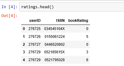

评分分布

评分分布非常不均衡，绝大部分都是0。

plt.rc("font", size=15)ratings.bookRating.value_counts(sort=False).plot(kind='bar')plt.title('Rating Distribution\n')plt.xlabel('Rating')plt.ylabel('Count')plt.savefig('system1.png', bbox_inches='tight')plt.show()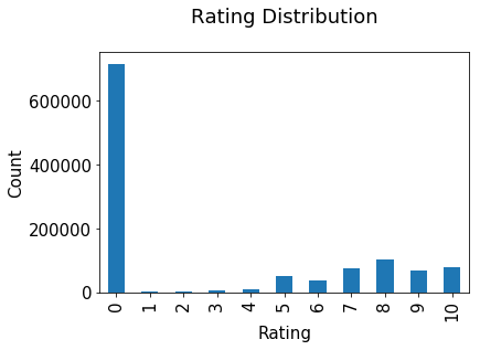

图书数据

图书数据集提供了很多细节，它包含了271360条记录，有 ISBN, book title, book author, publisher 等8个字段。

print(books.shape)print(list(books.columns))(271360, 8)['ISBN', 'bookTitle', 'bookAuthor', 'yearOfPublication', 'publisher', 'imageUrlS', 'imageUrlM', 'imageUrlL']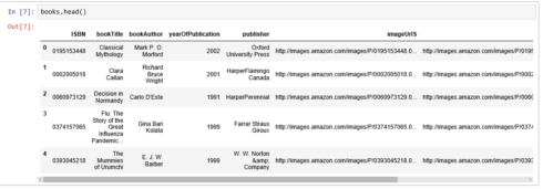

读者数据

这个数据集提供了读者的地域信息，有 user id, location, 和 age 3个字段，共278858条记录。

print(users.shape)print(list(users.columns))(278858, 3)['userID', 'Location', 'Age']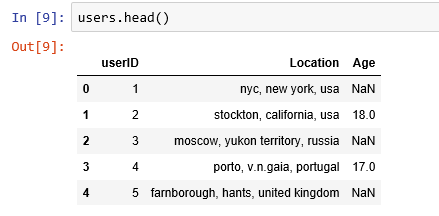

年龄分布

最活跃的用户大多20-30岁。

users.Age.hist(bins=[0, 10, 20, 30, 40, 50, 100])plt.title('Age Distribution\n')plt.xlabel('Age')plt.ylabel('Count')plt.savefig('system2.png', bbox_inches='tight')plt.show()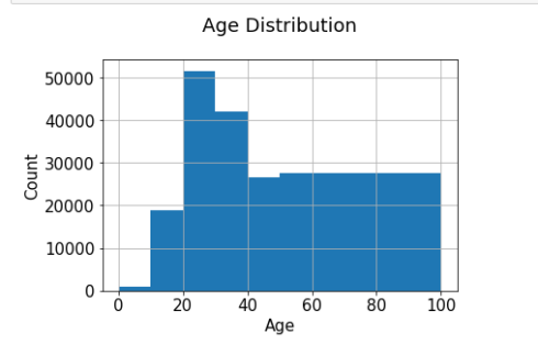

基于评分计数的推荐

rating_count = pd.DataFrame(ratings.groupby('ISBN')['bookRating'].count())rating_count.sort_values('bookRating', ascending=False).head()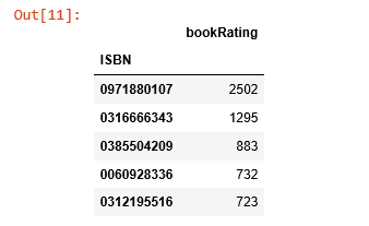

ISBN 号为0971880107的书籍收到了最多的评分，让我们看看这是本什么书，再探索下排名前5的书长什么样。

most_rated_books = pd.DataFrame(['0971880107', '0316666343', '0385504209', '0060928336', '0312195516'], index=np.arange(5), columns = ['ISBN'])most_rated_books_summary = pd.merge(most_rated_books, books, on='ISBN')most_rated_books_summary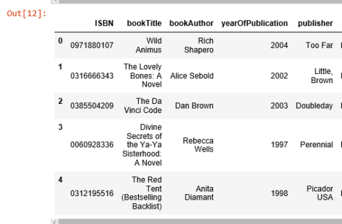

被评分次数最多的书是 Rich Shapero 的 “Wild Animus”，并且排名前5的图书都是小说。表明小说更受欢迎，并且容易收到评分。如果有人喜欢“The Lovely Bones: A Novel”, 那么我们应该向他/她推荐 “Wild Animus”。

基于相关性的推荐

我们使用皮尔森相关系数来衡量两个变量间的线性相关程度，本例中就研究两本图书评分的相关性。

首先，我们要计算平均评分和每本书收到的评分个数。

average_rating = pd.DataFrame(ratings.groupby('ISBN')['bookRating'].mean())average_rating['ratingCount'] = pd.DataFrame(ratings.groupby('ISBN')['bookRating'].count())average_rating.sort_values('ratingCount', ascending=False).head()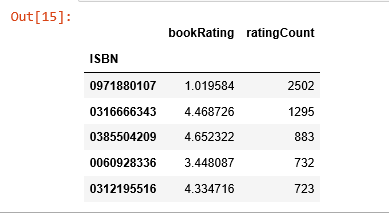

观测值：在这个图书数据集里，收到最多评分的书完全不是评分最高的那些。如果我们只以评分计数为推荐的条件，那么就错大发了。因此，我们需要一个更科学的系统。

为保证统计显著性，收到评分数少于100的图书和评分次数少于200次的读者都被排除在外。

counts1 = ratings['userID'].value_counts()ratings = ratings[ratings['userID'].isin(counts1[counts1 >= 200].index)]counts = ratings['bookRating'].value_counts()ratings = ratings[ratings['bookRating'].isin(counts[counts >= 100].index)]

评分矩阵

我们将评分转换为2维矩阵，这个矩阵会很稀疏因为不是每个读者都对每本书做了评分。

ratings_pivot = ratings.pivot(index='userID', columns='ISBN').bookRatinguserID = ratings_pivot.indexISBN = ratings_pivot.columnsprint(ratings_pivot.shape)ratings_pivot.head()(905, 207699)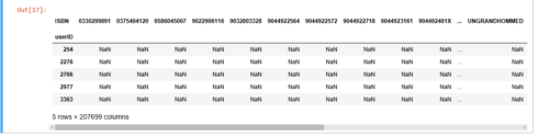

让我们来寻找被评分次数排名前2的书的相关性。

根据 维基百科，排名第二的书“The Lovely Bones: A Novel”是一个关于一位十几岁的小姑娘遭遇奸杀，在天堂观察家人艰辛生活的故事。

bones_ratings = ratings_pivot['0316666343']similar_to_bones = ratings_pivot.corrwith(bones_ratings)corr_bones = pd.DataFrame(similar_to_bones, columns=['pearsonR'])corr_bones.dropna(inplace=True)corr_summary = corr_bones.join(average_rating['ratingCount'])corr_summary[corr_summary['ratingCount']>=300].sort_values('pearsonR', ascending=False).head(10)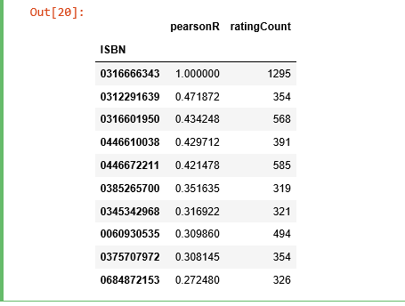

我们获取了所有书的 ISBN 号，现在我们需要查看它们的题目是否有信息。

books_corr_to_bones = pd.DataFrame(['0312291639', '0316601950', '0446610038', '0446672211', '0385265700', '0345342968', '0060930535', '0375707972', '0684872153'],                                   index=np.arange(9), columns=['ISBN'])corr_books = pd.merge(books_corr_to_bones, books, on='ISBN')corr_books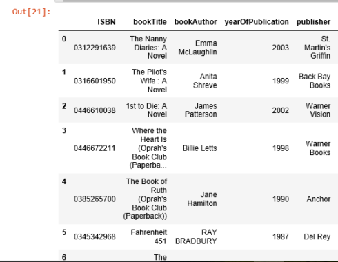

我们从高度相关的书籍列表中选取3本书，“The Nanny Diaries: A Novel”, “The Pilot’s Wife: A Novel” 和 “Where the Heart is”。
“The Nanny Diaries” 从保姆的视角讽刺了曼哈顿的上层社会。

“The Pilot’s Wife”和“The Lovely Bones”的作者是同一个人，作为非正式三部曲的最后一部，这个故事被设置在新罕布什尔州海岸的一个曾经是修道院的大型海滨别墅中。

“Where the Heart Is” 详细描述了美国低收入和寄养儿童的苦难。

这三本书听起来和“The Lovely Bones”有很高的相关性，看起来基于相关性的推荐系统起作用了。

使用基于 KNN 的协同滤波

KNN是一个用来基于共同图书评分以发现相似读者间聚类状况的机器学习算法，并且可以基于距离最近的 k 个邻居的平均评分来进行预测。举个例子，我们先看看评分矩阵，该矩阵每一行是一本书每一列是一个读者：

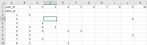
之后我们可以找到读者行为向量最为相似的k本图书，本例中 id = 5 的图书的最近邻的 id 为 [7, 4, 8, …]，现在让我们把这个方法用到推荐系统上。

这次我们只关注那些最为流行的图书，需要先对图书在评分这一维度上做些统计工作。

combine_book_rating = pd.merge(ratings, books, on='ISBN')columns = ['yearOfPublication', 'publisher', 'bookAuthor', 'imageUrlS', 'imageUrlM', 'imageUrlL']combine_book_rating = combine_book_rating.drop(columns, axis=1)combine_book_rating.head()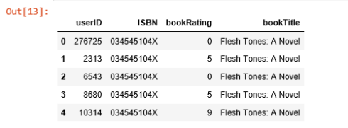

之后我们按照图书标题分组，并新增一列存储总的被评分次数。

combine_book_rating = combine_book_rating.dropna(axis = 0, subset = ['bookTitle'])book_ratingCount = (combine_book_rating.     groupby(by = ['bookTitle'])['bookRating'].     count().     reset_index().     rename(columns = {'bookRating': 'totalRatingCount'})     [['bookTitle', 'totalRatingCount']]    )book_ratingCount.head()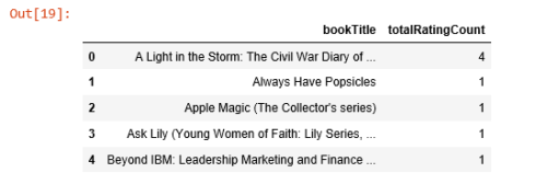

之后就可以筛选出最流行的书，把那些流传度不广的过滤掉。

rating_with_totalRatingCount = combine_book_rating.merge(book_ratingCount, left_on = 'bookTitle', right_on = 'bookTitle', how = 'left')rating_with_totalRatingCount.head()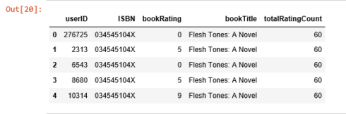

让我们看看这些统计量：

pd.set_option('display.float_format', lambda x: '%.3f' % x)print(book_ratingCount['totalRatingCount'].describe())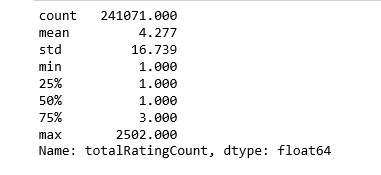

处在中位数位置的数就只被评分一次，让我们再看看头部的分布：

print(book_ratingCount['totalRatingCount'].quantile(np.arange(.9, 1, .01)))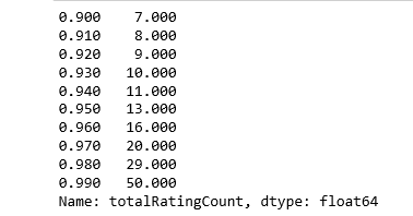

约有1%的书收到了超过50次的评分，由于数据集内记录众多，我们就截取头部1%的图书来建模，得到大概2713本书。

popularity_threshold = 50rating_popular_book = rating_with_totalRatingCount.query('totalRatingCount >= @popularity_threshold')rating_popular_book.head()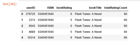

只保留美国和加拿大的读者

为了加快计算速度并节约内存，我只选取读者数据集中位于美国和加拿大的数据，然后把这个子集和之前得到的评分数据集合并。

combined = rating_popular_book.merge(users, left_on = 'userID', right_on = 'userID', how = 'left')us_canada_user_rating = combined[combined['Location'].str.contains("usa|canada")]us_canada_user_rating=us_canada_user_rating.drop('Age', axis=1)us_canada_user_rating.head()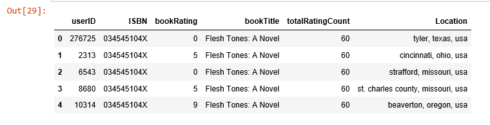

应用kNN

我们把数据表转化为一个二维矩阵，并把缺失值用0填充（因为要计算评分向量间的距离）。之后我们把矩阵中的评分数据转化伪scipy库中的稀疏矩阵来提升计算效率。

寻找近邻

我们使用sklean.neighbors这一无监督算法来寻找近邻，设定“metric=cosine”使得该算法基于余弦值来衡量相似度，最后我们再拟合模型。

us_canada_user_rating_pivot = us_canada_user_rating.pivot(index = 'bookTitle', columns = 'userID', values = 'bookRating').fillna(0)us_canada_user_rating_matrix = csr_matrix(us_canada_user_rating_pivot.values)from sklearn.neighbors import NearestNeighborsmodel_knn = NearestNeighbors(metric = 'cosine', algorithm = 'brute')model_knn.fit(us_canada_user_rating_matrix)NearestNeighbors(algorithm='brute', leaf_size=30, metric='cosine',         metric_params=None, n_jobs=1, n_neighbors=5, p=2, radius=1.0)

测试模型并做些推荐

这一步骤，kNN算法会计算距离作为实例间的近似度，然后找到实例的近邻，用近邻类别中的多数类对其进行分类。

query_index = np.random.choice(us_canada_user_rating_pivot.shape[0])distances, indices = model_knn.kneighbors(us_canada_user_rating_pivot.iloc[query_index, :].reshape(1, -1), n_neighbors = 6)for i in range(0, len(distances.flatten())):    if i == 0:        print('Recommendations for {0}:\n'.format(us_canada_user_rating_pivot.index[query_index]))    else:        print('{0}: {1}, with distance of {2}:'.format(i, us_canada_user_rating_pivot.index[indices.flatten()[i]], distances.flatten()[i]))Recommendations for the Green Mile: Coffey's Hands (Green Mile Series):1: The Green Mile: Night Journey (Green Mile Series), with distance of 0.26063737394209996:2: The Green Mile: The Mouse on the Mile (Green Mile Series), with distance of 0.2911623754404248:3: The Green Mile: The Bad Death of Eduard Delacroix (Green Mile Series), with distance of 0.2959542871302775:4: The Two Dead Girls (Green Mile Series), with distance of 0.30596709534565514:5: The Green Mile: Coffey on the Mile (Green Mile Series), with distance of 0.37646848777592923:

完美！Green Mile 系列图书就该逐一被推荐。

使用矩阵分解进行协同滤波

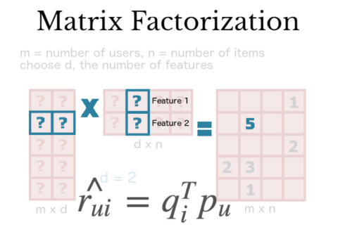
矩阵分解是一种常用的数学工具，这一技术非常有用，因为它使得用户可以发现读者和用户间的潜在交互特征。

本例我们将使用SVD分解，这是一种发现潜在因子的常用方法。

与kNN类似，我们把美国和加拿大读者的评分表转换为二维矩阵（命名为效用矩阵）并把缺失值用0填充。

us_canada_user_rating_pivot2 = us_canada_user_rating.pivot(index = 'userID', columns = 'bookTitle', values = 'bookRating').fillna(0)us_canada_user_rating_pivot2.head()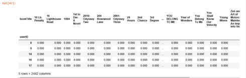

之后我们将效用矩阵转置，每行是图书标题，每列是读者ID。用 TruncatedSVD 对其进行分解之后，我们出于降维的目的拟合模型。由于我们要保留图书标题，现在这一过程是针对矩阵的列进行的。我们设定 n_components = 12 来寻找12个潜在变量，这样我们的维度就从40017 X 2442 降至 2442 X 12。

us_canada_user_rating_pivot2.shape(40017, 2442)

X = us_canada_user_rating_pivot2.values.TX.shape(2442, 40017)

import sklearnfrom sklearn.decomposition import TruncatedSVDSVD = TruncatedSVD(n_components=12, random_state=17)matrix = SVD.fit_transform(X)matrix.shape(2442, 12)

在最终的矩阵中，我们计算了每两本书之间的皮尔森相关系数，为了比较它与kNN的效果，我们以 “The Green Mile: Coffey’s Hands (Green Mile Series)”作为案例，寻找和他相关系数（0.9到1之间）最高的书。

import warningswarnings.filterwarnings("ignore",category =RuntimeWarning)corr = np.corrcoef(matrix)corr.shape(2442, 2442)

us_canada_book_title = us_canada_user_rating_pivot2.columnsus_canada_book_list = list(us_canada_book_title)coffey_hands = us_canada_book_list.index("The Green Mile: Coffey's Hands (Green Mile Series)")print(coffey_hands)1906

看到了吧！

corr_coffey_hands  = corr[coffey_hands]list(us_canada_book_title[(corr_coffey_hands0.9)])['Needful Things', 'The Bachman Books: Rage, the Long Walk, Roadwork, the Running Man',s 'The Green Mile: Coffey on the Mile (Green Mile Series)', 'The Green Mile: Night Journey (Green Mile Series)', 'The Green Mile: The Bad Death of Eduard Delacroix (Green Mile Series)', 'The Green Mile: The Mouse on the Mile (Green Mile Series)', 'The Shining', 'The Two Dead Girls (Green Mile Series)']

不谦虚地说，这个系统可以打败亚马逊的推荐系统，你觉得呢?

参考文献：

Music RecommendationsohAI

原文链接