scipy-图像操作

参考：
1、https://docs.scipy.org/doc/scipy/reference/ndimage.html#module-scipy.ndimage
2、http://scipy-lectures.github.com/advanced/image_processing/index.html
3、http://blog.csdn.net/zt_706/article/details/11476433

这个教程中使用的工具：

• numpy：基本数组操作
• scipy：scipy.ndimage子模块致力于图像处理(n维图像)。参见http://docs.scipy.org/doc/scipy/reference/tutorial/ndimage.html

from scipy import ndimage

• 一些例子用到了使用np.array的特殊的工具箱：
  
  • Scikit Image
  • scikit-learn

图像中的常见问题有：

• 输入/输出：呈现图像
• 基本操作：裁剪、翻转、旋转、比例缩放……
• 图像滤镜：消噪，锐化
• 图像分割：不同对应对象的像素标记

更有力和完整的模块：

• OpenCV (Python绑定)
• CellProfiler
• ITK,Python绑定
• 更多……

1、打开和读写图像文件

将一个数组写入文件：

In [1]: from scipy import miscIn [2]: l = misc.lena()In [3]: misc.imsave('lena.png', l)  # uses the Image module (PIL)In [4]: import pylab as plIn [5]: pl.imshow(l)Out[5]: <matplotlib.image.AxesImage at 0x4118110>

从一个图像文件创建数组：

import matplotlib.pyplot as pltfrom scipy import miscimport pylab as plimg1=misc.imread('Lenna.png',mode='L')img2=misc.imread('Lenna.png',mode='RGB')img3=misc.imread('Lenna.png',mode='RGBA')pl.imshow(img2,cmap='gray')pl.show()misc.imsave('lena.png',img2) # 保存# pl可以使用plt替换

或

from scipy import ndimagendimage.imread('lena.png',mode='L') # 加载灰度图ndimage.imread('lena.png', mode='RGB')  # 加载RGB图ndimage.imread('lena.png', mode='RGBA')  # 加载RGBA图

打开一个raw文件(相机， 3-D图像)

#!/usr/bin/env python3# -*- coding: UTF-8 -*-from scipy import miscimport numpy as npimport pylab as plimg=misc.imread('Lenna.png',mode='L')# print(img.dtype) # uint8img.tofile('lena.raw') # 创建一个raw文件lena_from_raw = np.fromfile('lena.raw',np.uint8) # 加载 lena.raw 文件print(lena_from_raw.shape)# lena_from_raw=np.reshape(lena_from_raw,[512,512])lena_from_raw.shape = (512, 512)pl.imshow(lena_from_raw,cmap='gray')pl.show()import osos.remove('lena.raw') # 删除文件

对于大数据，使用np.memmap进行内存映射：

#!/usr/bin/env python3# -*- coding: UTF-8 -*-from scipy import miscimport numpy as npimport pylab as plimg=misc.imread('Lenna.png',mode='RGB')# print(img.dtype) # uint8img.tofile('lena.raw') # 创建一个raw文件 保存成raw文件lena_memmap = np.memmap('lena.raw', dtype=np.uint8, shape=(512,512,3)) # 加载raw文件pl.imshow(lena_memmap,cmap='gray')pl.show()import osos.remove('lena.raw') # 删除文件

批量处理图像文件：

In [22]: for i in range(10):   ....:     im = np.random.random_integers(0, 255, 10000).reshape((100, 100))   ....:     misc.imsave('random_%02d.png' % i, im)   ....:     In [23]: from glob import globIn [24]: filelist = glob('random*.png')In [25]: filelist.sort()

2、呈现图像

使用matplotlib和imshow将图像呈现在matplotlib图像(figure)中：

#!/usr/bin/env python3# -*- coding: UTF-8 -*-from scipy import miscimport numpy as npimport pylab as plimport matplotlib.pyplot as pltimg=misc.imread('Lenna.png',mode='L')plt.imshow(img,cmap=plt.cm.gray)plt.imshow(img, cmap='gray', vmin=30, vmax=200) # 设置最大最小之增加对比# 更好地观察强度变化，使用interpolate=‘nearest’plt.imshow(img[200:220, 200:220], cmap=plt.cm.gray, interpolation='nearest')plt.axis('off')  # 移除axes和ticksplt.contour(img, [60, 211])  # 绘制等高线plt.show()# ---将plt换成pl-----------------------------------------------------------------pl.imshow(img,cmap=plt.cm.gray)pl.imshow(img, cmap='gray', vmin=30, vmax=200) # 设置最大最小之增加对比# 更好地观察强度变化，使用interpolate=‘nearest’pl.imshow(img[200:220, 200:220], cmap=pl.cm.gray, interpolation='nearest')pl.axis('off')  # 移除axes和tickspl.contour(img, [60, 211])  # 绘制等高线pl.show()

其它包有时使用图形工具箱来可视化(GTK，Qt)

#!/usr/bin/env python3# -*- coding: UTF-8 -*-from scipy import miscimport numpy as npimport skimage.io as im_ioimg=misc.imread('Lenna.png',mode='L')im_io.use_plugin('gtk', 'imshow')im_io.imshow(img)im_io.show()

3-D可视化：Mayavi

参见可用Mayavi进行3-D绘图和体积数据

• 图形平面工具
• 等值面
• ……

3、基本操作

图像是数组（numpy array）。

>>> lena = misc.lena()>>> lena[0, 40]166>>> # Slicing>>> lena[10:13, 20:23]array([[158, 156, 157],[157, 155, 155],[157, 157, 158]])>>> lena[100:120] = 255>>>>>> lx, ly = lena.shape>>> X, Y = np.ogrid[0:lx, 0:ly]>>> mask = (X - lx/2)**2 + (Y - ly/2)**2 > lx*ly/4>>> # Masks>>> lena[mask] = 0>>> # Fancy indexing>>> lena[range(400), range(400)] = 255

统计信息

#!/usr/bin/env python3# -*- coding: UTF-8 -*-from scipy import miscimport numpy as npimport pylab as plimport matplotlib.pyplot as pltimport cv2lena=misc.imread('Lenna.png',mode='L') # 数据类型 numpy arraylena.mean() # 平均值lena.max() # 最大值lena.min() # 最小值# 图像直方图# 1、使用np.histogramhist, bins = np.histogram(lena.ravel(), bins=256, range=[0,256],normed=True)plt.plot(hist)plt.legend(loc='best')plt.show()# 2、使用plt.histplt.hist(lena.ravel(),256,[0,256]); plt.show()# 3、使用opencvhist_full = cv2.calcHist([lena],[0],None,[256],[0,256])plt.plot(hist_full)plt.xlim([0,256])plt.show()

几何转换

#!/usr/bin/env python3# -*- coding: UTF-8 -*-from scipy import miscimport numpy as npimport scipyimport pylab as plimport matplotlib.pyplot as pltimport cv2lena=misc.imread('Lenna.png',mode='L') # 数据类型 numpy arraylx, ly = lena.shape# 裁剪crop_lena = lena[lx/4:-lx/4, ly/4:-ly/4]# 上下翻转flip_ud_lena = np.flipud(lena)# 左右翻转flip_lr_lena = np.fliplr(lena)# 任意角度旋转rotate_lena = ndimage.rotate(lena, 45)rotate_lena_noreshape = ndimage.rotate(lena, 45, reshape=False) # 不改变原图大小# 任意缩放zoomed_lena = ndimage.zoom(lena, 2) # 放大2倍zoomed_lena2 = ndimage.zoom(lena, 0.5) # 缩小1/2倍

4、图像滤镜

局部滤镜
：用相邻像素值的函数替代当前像素的值。

相邻：方形(指定大小)，圆形， 或者更多复杂的结构元素。

模糊/平滑

scipy.ndimage中的高斯滤镜：

>>> from scipy import misc>>> from scipy import ndimage>>> lena = misc.lena()>>> blurred_lena = ndimage.gaussian_filter(lena, sigma=3)>>> very_blurred = ndimage.gaussian_filter(lena, sigma=5)

均匀滤镜

>>> local_mean = ndimage.uniform_filter(lena, size=11)

锐化

锐化模糊图像：

#!/usr/bin/env python3# -*- coding: UTF-8 -*-from scipy import miscimport pylab as plfrom scipy import ndimagelena=misc.imread('Lenna.png',mode='L') # 数据类型 numpy array# 锐化模糊图像blurred_l = ndimage.gaussian_filter(lena, 3)# 通过增加拉普拉斯近似增加边缘权重filter_blurred_l = ndimage.gaussian_filter(blurred_l, 1)alpha = 30sharpened = blurred_l + alpha * (blurred_l - filter_blurred_l)pl.subplot(131),pl.imshow(blurred_l,cmap='gray'),pl.axis('off'),pl.title('blurred_l')pl.subplot(132),pl.imshow(filter_blurred_l,cmap='gray'),pl.axis('off'),pl.title('filter_blurred_l')pl.subplot(133),pl.imshow(sharpened,cmap='gray'),pl.axis('off'),pl.title('sharpened')pl.show()

消噪

#!/usr/bin/env python3# -*- coding: UTF-8 -*-from scipy import miscimport pylab as plfrom scipy import ndimageimport numpy as nplena=misc.imread('Lenna.png',mode='L') # 数据类型 numpy array# 向lena增加噪声l = lena[230:310, 210:350]noisy = l + 0.4*l.std()*np.random.random(l.shape)# 高斯滤镜平滑掉噪声……还有边缘gauss_denoised = ndimage.gaussian_filter(noisy, 2)# 大多局部线性各向同性滤镜都模糊图像(ndimage.uniform_filter)unif_denoised=ndimage.uniform_filter(noisy,2)# 中值滤镜更好地保留边缘med_denoised = ndimage.median_filter(noisy, 3)pl.subplot(141),pl.imshow(noisy,cmap='gray'),pl.axis('off'),pl.title('noisy')pl.subplot(142),pl.imshow(gauss_denoised,cmap='gray'),pl.axis('off'),pl.title('gauss_denoised')pl.subplot(143),pl.imshow(unif_denoised,cmap='gray'),pl.axis('off'),pl.title('unif_denoised')pl.subplot(144),pl.imshow(med_denoised,cmap='gray'),pl.axis('off'),pl.title('med_denoised')pl.show()

其它排序滤波器：
ndimage.maximum_filter,ndimage.percentile_filter

其它局部非线性滤波器：
维纳滤波器(scipy.signal.wiener)等

非局部滤波器

总变差(TV)消噪。找到新的图像让图像的总变差(正态L1梯度的积分)变得最小，当接近测量图像时

#!/usr/bin/env python3# -*- coding: UTF-8 -*-from scipy import miscimport pylab as plfrom scipy import ndimageimport numpy as np# from skimage.filter import denoise_tv_bregman,denoise_tv_chambollefrom skimage.restoration import denoise_tv_bregman,denoise_tv_chambollelena=misc.imread('Lenna.png',mode='L') # 数据类型 numpy array# 向lena增加噪声l = lena[230:310, 210:350]noisy = l + 0.4*l.std()*np.random.random(l.shape)tv_denoised_b = denoise_tv_bregman(noisy, weight=10)tv_denoised_c = denoise_tv_chambolle(noisy, weight=10)ax=pl.figure()ax.add_subplot(131),pl.imshow(noisy,cmap='gray'),pl.axis('off'),pl.title('noisy')pl.show()# pl.subplot(131),pl.imshow(noisy,cmap='gray'),pl.axis('off'),pl.title('noisy')# pl.subplot(132),pl.imshow(tv_denoised_b,cmap='gray'),pl.axis('off'),pl.title('tv_denoised_b')# pl.subplot(133),pl.imshow(tv_denoised_c,cmap='gray'),pl.axis('off'),pl.title('tv_denoised_c')## pl.show()

5、数学形态学

结构元素

>>> el = ndimage.generate_binary_structure(2, 1)>>> elarray([[False,  True, False],       [ True,  True,  True],       [False,  True, False]], dtype=bool)>>> el.astype(np.int)array([[0, 1, 0],       [1, 1, 1],       [0, 1, 0]])

腐蚀 = 最小化滤镜。用结构元素覆盖的像素的最小值替代一个像素值：

>>> a = np.zeros((7,7), dtype=np.int)>>> a[1:6, 2:5] = 1>>> aarray([[0, 0, 0, 0, 0, 0, 0],       [0, 0, 1, 1, 1, 0, 0],       [0, 0, 1, 1, 1, 0, 0],       [0, 0, 1, 1, 1, 0, 0],       [0, 0, 1, 1, 1, 0, 0],       [0, 0, 1, 1, 1, 0, 0],       [0, 0, 0, 0, 0, 0, 0]])>>> ndimage.binary_erosion(a).astype(a.dtype)array([[0, 0, 0, 0, 0, 0, 0],       [0, 0, 0, 0, 0, 0, 0],       [0, 0, 0, 1, 0, 0, 0],       [0, 0, 0, 1, 0, 0, 0],       [0, 0, 0, 1, 0, 0, 0],       [0, 0, 0, 0, 0, 0, 0],       [0, 0, 0, 0, 0, 0, 0]])>>> #Erosion removes objects smaller than the structure>>> ndimage.binary_erosion(a, structure=np.ones((5,5))).astype(a.dtype)array([[0, 0, 0, 0, 0, 0, 0],       [0, 0, 0, 0, 0, 0, 0],       [0, 0, 0, 0, 0, 0, 0],       [0, 0, 0, 0, 0, 0, 0],       [0, 0, 0, 0, 0, 0, 0],       [0, 0, 0, 0, 0, 0, 0],       [0, 0, 0, 0, 0, 0, 0]])

膨胀：最大化滤镜:

>>> a = np.zeros((5, 5))>>> a[2, 2] = 1>>> aarray([[ 0.,  0.,  0.,  0.,  0.],       [ 0.,  0.,  0.,  0.,  0.],       [ 0.,  0.,  1.,  0.,  0.],       [ 0.,  0.,  0.,  0.,  0.],       [ 0.,  0.,  0.,  0.,  0.]])>>> ndimage.binary_dilation(a).astype(a.dtype)array([[ 0.,  0.,  0.,  0.,  0.],       [ 0.,  0.,  1.,  0.,  0.],       [ 0.,  1.,  1.,  1.,  0.],       [ 0.,  0.,  1.,  0.,  0.],       [ 0.,  0.,  0.,  0.,  0.]])

对灰度值图像也有效

>>> np.random.seed(2)>>> x, y = (63*np.random.random((2, 8))).astype(np.int)>>> im[x, y] = np.arange(8)>>> bigger_points = ndimage.grey_dilation(im, size=(5, 5), structure=np.ones((5, 5)))>>> square = np.zeros((16, 16))>>> square[4:-4, 4:-4] = 1>>> dist = ndimage.distance_transform_bf(square)>>> dilate_dist = ndimage.grey_dilation(dist, size=(3, 3), \...         structure=np.ones((3, 3)))

开操作：腐蚀+膨胀
应用：移除噪声

>>> square = np.zeros((32, 32))>>> square[10:-10, 10:-10] = 1>>> np.random.seed(2)>>> x, y = (32*np.random.random((2, 20))).astype(np.int)>>> square[x, y] = 1>>> open_square = ndimage.binary_opening(square)>>> eroded_square = ndimage.binary_erosion(square)>>> reconstruction = ndimage.binary_propagation(eroded_square, mask=square)

示例代码

闭操作：膨胀+腐蚀

许多其它数学分形：击中(hit)和击不中(miss)变换，tophat等等。

6、特征提取

边缘检测

使用梯度操作(Sobel)来找到搞强度的变化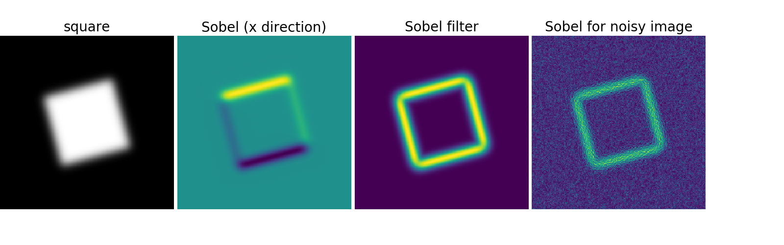

示例源码

canny滤镜

Canny滤镜可以从skimage中获取(文档)

>>> #from skimage.filter import canny>>> #or use module shipped with tutorial>>> im += 0.1*np.random.random(im.shape)>>> edges = canny(im, 1, 0.4, 0.2) # not enough smoothing>>> edges = canny(im, 3, 0.3, 0.2) # better parameters

示例代码

分割

基于直方图的分割(没有空间信息)

 >>> n = 10  >>> l = 256  >>> im = np.zeros((l, l))  >>> np.random.seed(1)  >>> points = l*np.random.random((2, n**2))  >>> im[(points[0]).astype(np.int), (points[1]).astype(np.int)] = 1  >>> im = ndimage.gaussian_filter(im, sigma=l/(4.*n))  >>> mask = (im > im.mean()).astype(np.float)  >>> mask += 0.1 * im  >>> img = mask + 0.2*np.random.randn(*mask.shape)  >>> hist, bin_edges = np.histogram(img, bins=60)  >>> bin_centers = 0.5*(bin_edges[:-1] + bin_edges[1:])  >>> binary_img = img > 0.5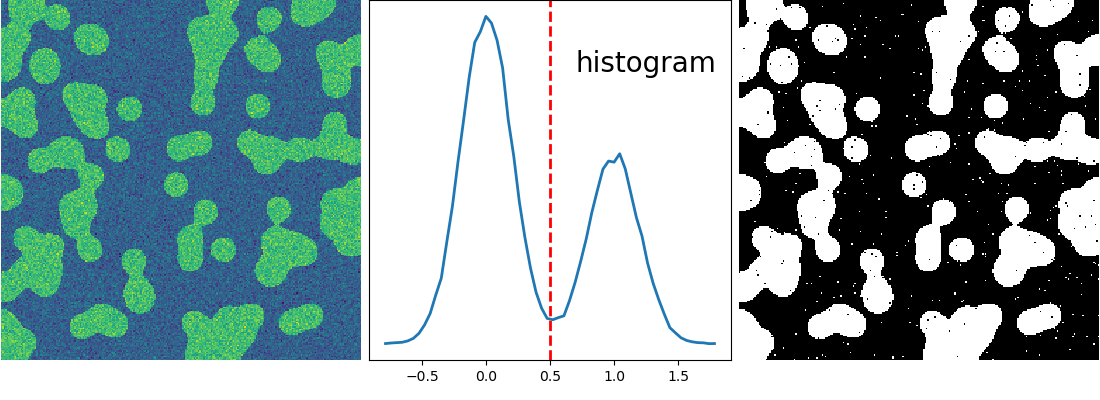

示例代码

自动阈值：使用高斯混合模型

>>> mask = (im > im.mean()).astype(np.float)>>> mask += 0.1 * im>>> img = mask + 0.3*np.random.randn(*mask.shape)>>> from sklearn.mixture import GMM>>> classif = GMM(n_components=2)>>> classif.fit(img.reshape((img.size, 1))) GMM(...)>>> classif.means_array([[ 0.9353155 ],       [-0.02966039]])>>> np.sqrt(classif.covars_).ravel()array([ 0.35074631,  0.28225327])>>> classif.weights_array([ 0.40989799,  0.59010201])>>> threshold = np.mean(classif.means_)>>> binary_img = img > threshold

使用数学形态学来清理结果：

>>> # Remove small white regions>>> open_img = ndimage.binary_opening(binary_img)>>> # Remove small black hole>>> close_img = ndimage.binary_closing(open_img)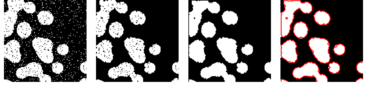

示例源码

其他略

参考：http://scipy-lectures.github.com/advanced/image_processing/index.html