k-means聚类算法python实现

来源：互联网发布：aria2 windows懒人包编辑：程序博客网时间：2024/05/21 07:46

来自：

https://www.cnblogs.com/MrLJC/p/4127553.html

K-means聚类算法

算法优缺点：

优点：容易实现
缺点：可能收敛到局部最小值，在大规模数据集上收敛较慢
使用数据类型：数值型数据

算法思想

k-means算法实际上就是通过计算不同样本间的距离来判断他们的相近关系的，相近的就会放到同一个类别中去。

1.首先我们需要选择一个k值，也就是我们希望把数据分成多少类，这里k值的选择对结果的影响很大，Ng的课说的选择方法有两种一种是elbow method，简单的说就是根据聚类的结果和k的函数关系判断k为多少的时候效果最好。另一种则是根据具体的需求确定，比如说进行衬衫尺寸的聚类你可能就会考虑分成三类（L,M,S）等

2.然后我们需要选择最初的聚类点（或者叫质心），这里的选择一般是随机选择的，代码中的是在数据范围内随机选择，另一种是随机选择数据中的点。这些点的选择会很大程度上影响到最终的结果，也就是说运气不好的话就到局部最小值去了。这里有两种处理方法，一种是多次取均值，另一种则是后面的改进算法（bisecting K-means）

3.终于我们开始进入正题了，接下来我们会把数据集中所有的点都计算下与这些质心的距离，把它们分到离它们质心最近的那一类中去。完成后我们则需要将每个簇算出平均值，用这个点作为新的质心。反复重复这两步，直到收敛我们就得到了最终的结果。

函数

loadDataSet(fileName)
从文件中读取数据集
distEclud(vecA, vecB)
计算距离，这里用的是欧氏距离，当然其他合理的距离都是可以的
randCent(dataSet, k)
随机生成初始的质心，这里是虽具选取数据范围内的点
kMeans(dataSet, k, distMeas=distEclud, createCent=randCent)
kmeans算法，输入数据和k值。后面两个事可选的距离计算方式和初始质心的选择方式
show(dataSet, k, centroids, clusterAssment)
可视化结果

 1 #coding=utf-8 2 from numpy import * 3  4 def loadDataSet(fileName): 5     dataMat = [] 6     fr = open(fileName) 7     for line in fr.readlines(): 8         curLine = line.strip().split('\t') 9         fltLine = map(float, curLine)10         dataMat.append(fltLine)11     return dataMat12     13 #计算两个向量的距离，用的是欧几里得距离14 def distEclud(vecA, vecB):15     return sqrt(sum(power(vecA - vecB, 2)))16 17 #随机生成初始的质心（ng的课说的初始方式是随机选K个点）    18 def randCent(dataSet, k):19     n = shape(dataSet)[1]20     centroids = mat(zeros((k,n)))21     for j in range(n):22         minJ = min(dataSet[:,j])23         rangeJ = float(max(array(dataSet)[:,j]) - minJ)24         centroids[:,j] = minJ + rangeJ * random.rand(k,1)25     return centroids26     27 def kMeans(dataSet, k, distMeas=distEclud, createCent=randCent):28     m = shape(dataSet)[0]29     clusterAssment = mat(zeros((m,2)))#create mat to assign data points 30                                       #to a centroid, also holds SE of each point31     centroids = createCent(dataSet, k)32     clusterChanged = True33     while clusterChanged:34         clusterChanged = False35         for i in range(m):#for each data point assign it to the closest centroid36             minDist = inf37             minIndex = -138             for j in range(k):39                 distJI = distMeas(centroids[j,:],dataSet[i,:])40                 if distJI < minDist:41                     minDist = distJI; minIndex = j42             if clusterAssment[i,0] != minIndex: 43                 clusterChanged = True44             clusterAssment[i,:] = minIndex,minDist**245         print centroids46         for cent in range(k):#recalculate centroids47             ptsInClust = dataSet[nonzero(clusterAssment[:,0].A==cent)[0]]#get all the point in this cluster48             centroids[cent,:] = mean(ptsInClust, axis=0) #assign centroid to mean 49     return centroids, clusterAssment50     51 def show(dataSet, k, centroids, clusterAssment):52     from matplotlib import pyplot as plt  53     numSamples, dim = dataSet.shape  54     mark = ['or', 'ob', 'og', 'ok', '^r', '+r', 'sr', 'dr', '<r', 'pr']  55     for i in xrange(numSamples):  56         markIndex = int(clusterAssment[i, 0])  57         plt.plot(dataSet[i, 0], dataSet[i, 1], mark[markIndex])  58     mark = ['Dr', 'Db', 'Dg', 'Dk', '^b', '+b', 'sb', 'db', '<b', 'pb']  59     for i in range(k):  60         plt.plot(centroids[i, 0], centroids[i, 1], mark[i], markersize = 12)  61     plt.show()62       63 def main():64     dataMat = mat(loadDataSet('testSet.txt'))65     myCentroids, clustAssing= kMeans(dataMat,4)66     print myCentroids67     show(dataMat, 4, myCentroids, clustAssing)  68     69     70 if __name__ == '__main__':71     main()

这里是聚类结果，还是很不错的啦

但是有时候也会收敛到局部最小值，就像下面这样，就是不幸收敛到局部最优了

k 值选择：https://www.cnblogs.com/wuchuanying/p/6264025.html

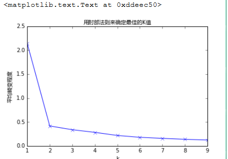
# K的选择：肘部法则

如果问题中没有指定的值，可以通过肘部法则这一技术来估计聚类数量。肘部法则会把不同值的
成本函数值画出来。随着值的增大，平均畸变程度会减小；每个类包含的样本数会减少，于是样本
离其重心会更近。但是，随着值继续增大，平均畸变程度的改善效果会不断减低。值增大过程
中，畸变程度的改善效果下降幅度最大的位置对应的值就是肘部。

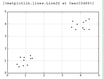
import numpy as npimport matplotlib.pyplot as plt%matplotlib inline#随机生成一个实数，范围在（0.5,1.5）之间cluster1=np.random.uniform(0.5,1.5,(2,10))cluster2=np.random.uniform(3.5,4.5,(2,10))#hstack拼接操作X=np.hstack((cluster1,cluster2)).Tplt.figure()plt.axis([0,5,0,5])plt.grid(True)plt.plot(X[:,0],X[:,1],'k.')

%matplotlib inlineimport matplotlib.pyplot as pltfrom matplotlib.font_manager import FontPropertiesfont = FontProperties(fname=r"c:\windows\fonts\msyh.ttc", size=10)

#coding:utf-8#我们计算K值从1到10对应的平均畸变程度：from sklearn.cluster import KMeans#用scipy求解距离from scipy.spatial.distance import cdistK=range(1,10)meandistortions=[]for k in K:    kmeans=KMeans(n_clusters=k)    kmeans.fit(X)    meandistortions.append(sum(np.min(            cdist(X,kmeans.cluster_centers_,                 'euclidean'),axis=1))/X.shape[0])plt.plot(K,meandistortions,'bx-')plt.xlabel('k')plt.ylabel(u'平均畸变程度',fontproperties=font)plt.title(u'用肘部法则来确定最佳的K值',fontproperties=font)

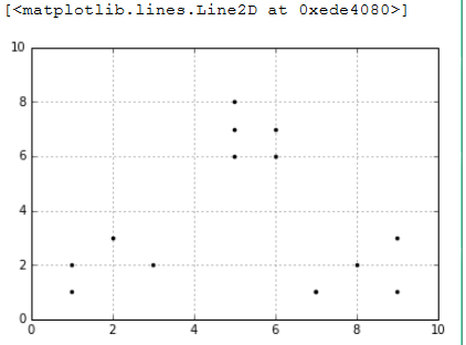
import numpy as npx1 = np.array([1, 2, 3, 1, 5, 6, 5, 5, 6, 7, 8, 9, 7, 9])x2 = np.array([1, 3, 2, 2, 8, 6, 7, 6, 7, 1, 2, 1, 1, 3])X=np.array(list(zip(x1,x2))).reshape(len(x1),2)plt.figure()plt.axis([0,10,0,10])plt.grid(True)plt.plot(X[:,0],X[:,1],'k.')

from sklearn.cluster import KMeansfrom scipy.spatial.distance import cdistK=range(1,10)meandistortions=[]for k in K:    kmeans=KMeans(n_clusters=k)    kmeans.fit(X)    meandistortions.append(sum(np.min(cdist(            X,kmeans.cluster_centers_,"euclidean"),axis=1))/X.shape[0])plt.plot(K,meandistortions,'bx-')plt.xlabel('k')plt.ylabel(u'平均畸变程度',fontproperties=font)plt.title(u'用肘部法则来确定最佳的K值',fontproperties=font)

# 聚类效果的评价
#### 轮廓系数（Silhouette Coefficient）:s =ba/max(a, b)

import numpy as npfrom sklearn.cluster import KMeansfrom sklearn import metricsplt.figure(figsize=(8,10))plt.subplot(3,2,1)x1 = np.array([1, 2, 3, 1, 5, 6, 5, 5, 6, 7, 8, 9, 7, 9])x2 = np.array([1, 3, 2, 2, 8, 6, 7, 6, 7, 1, 2, 1, 1, 3])X = np.array(list(zip(x1, x2))).reshape(len(x1), 2)plt.xlim([0,10])plt.ylim([0,10])plt.title(u'样本',fontproperties=font)plt.scatter(x1, x2)colors = ['b', 'g', 'r', 'c', 'm', 'y', 'k', 'b']markers = ['o', 's', 'D', 'v', '^', 'p', '*', '+']tests=[2,3,4,5,8]subplot_counter=1for t in tests:    subplot_counter+=1    plt.subplot(3,2,subplot_counter)    kmeans_model=KMeans(n_clusters=t).fit(X)#     print kmeans_model.labels_:每个点对应的标签值    for i,l in enumerate(kmeans_model.labels_):        plt.plot(x1[i],x2[i],color=colors[l],             marker=markers[l],ls='None')        plt.xlim([0,10])        plt.ylim([0,10])        plt.title(u'K = %s, 轮廓系数 = %.03f' %                   (t, metrics.silhouette_score                   (X, kmeans_model.labels_,metric='euclidean'))                  ,fontproperties=font)

# 图像向量化

import numpy as npfrom sklearn.cluster import KMeansfrom sklearn.utils import shuffleimport mahotas as mhoriginal_img=np.array(mh.imread('tree.bmp'),dtype=np.float64)/255original_dimensions=tuple(original_img.shape)width,height,depth=tuple(original_img.shape)image_flattend=np.reshape(original_img,(width*height,depth))print image_flattend.shapeimage_flattend

输出结果：

(102672L, 3L)

Out[96]:

array([[ 0.55686275,  0.57647059,  0.61960784],       [ 0.68235294,  0.70196078,  0.74117647],       [ 0.72156863,  0.7372549 ,  0.78039216],       ...,        [ 0.75686275,  0.63529412,  0.46666667],       [ 0.74117647,  0.61568627,  0.44705882],       [ 0.70588235,  0.57647059,  0.40784314]])

然后我们用K-Means算法在随机选择1000个颜色样本中建立64个类。每个类都可能是压缩调色板中的一种颜色

image_array_sample=shuffle(image_flattend,random_state=0)[:1000]image_array_sample.shapeestimator=KMeans(n_clusters=64,random_state=0)estimator.fit(image_array_sample)#之后，我们为原始图片的每个像素进行类的分配cluster_assignments=estimator.predict(image_flattend)print cluster_assignments.shapecluster_assignments

输出结果：

(102672L,)

Out[105]:

array([59, 39, 33, ..., 46,  8, 17])

#最后，我们建立通过压缩调色板和类分配结果创建压缩后的图片：compressed_palette = estimator.cluster_centers_compressed_img = np.zeros((width, height, compressed_palette.shape[1]))label_idx = 0for i in range(width):    for j in range(height):        compressed_img[i][j] = compressed_palette[cluster_assignments[label_idx]]        label_idx += 1plt.subplot(122)plt.title('Original Image')plt.imshow(original_img)plt.axis('off')plt.subplot(121)plt.title('Compressed Image')plt.imshow(compressed_img)plt.axis('off')plt.show()

阅读全文

0 0