BP算法从原理到python实现
来源:互联网 发布:mac程序文件夹在哪里 编辑:程序博客网 时间:2024/05/20 20:01
BP算法从原理到实践
Backpropagation算法的python实现
觉得有用的话,欢迎一起讨论相互学习~Follow Me
博主接触深度学习已经一段时间,近期在与别人进行讨论时,发现自己对于反向传播算法理解的并不是十分的透彻,现在想通过这篇博文缕清一下思路.自身才疏学浅欢迎各位批评指正.
参考文献
李宏毅深度学习视频
The original location of the code关于反向传播算法的用途在此不再赘述,这篇博文主要是理解形象化理解反向传播算法与python进行实践的.
一张图读懂反向传播算法

反向传播是一种有效率进行梯度下降的方法
- 在神经网络中,我们往往有很多参数,每一个神经元与另一个神经元的连接都有一个权重(weight),每一个神经元都有一个偏置(bias).在梯度下降减小loss function的值时我们会对所有的参数进行更新.
- 我们设所有的参数为
θ ,初始化的θ 记为θ0 .其经过梯度下降后的取值设为θ1,θ2,θ3...θn η 表示学习率,L(θ) 表示Lossfunction,∇ 表示梯度.
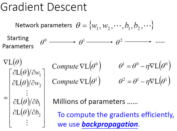
- 假设我们需要做语音辨识,有7-8层神经层,每层有1000个神经元,这时我们的梯度向量
∇L(θ) 是一个有上百万维度的向量,这时候我们使用反向传播算法有效率的计算参数的梯度下降值.
BP算法数学原理直观表示
Chain Rule 链式法则
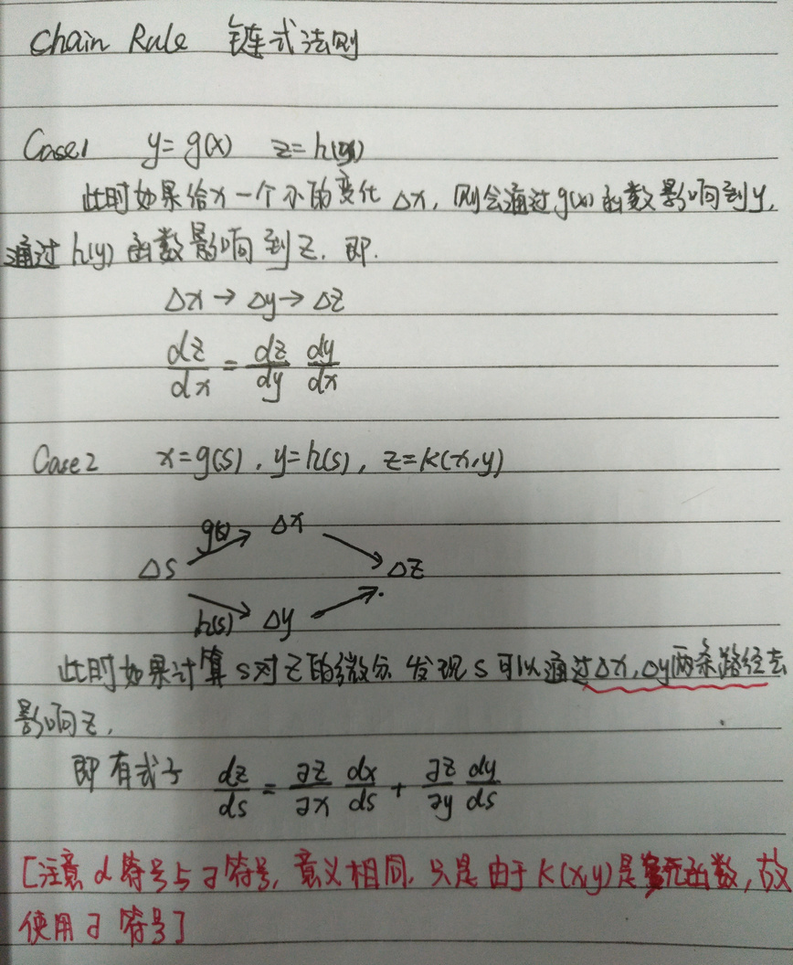
- 我们将训练数据的正确值(理想值)称为
y^ 而把模型的实际输出值记作y .Cost function是对于一个训练数据y和y^距离的函数 .则Lost function是所有训练数据的Cost function值的加和. - 即若我们想计算Loss function对w的偏导数,只要计算训练集上所有训练数据对w的偏导数之和即可.
Backpropagation 实现
- 假设我们取一个简单神经网络的输入层作考虑.


Forward pass前向传播
- 对于前向传播,[即前向传播中的连接输入值(也是连接中上一个神经元的输出值)即是激活函数对该边权值的偏导数]
∂z∂wn=Xn

也就是说只要我们算出每一个神经元的输出就能知道与其相连的边的cost function 对权值的偏微分.
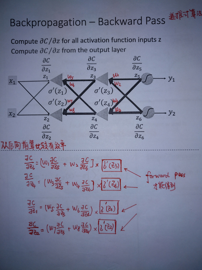
Backward pass反向传播
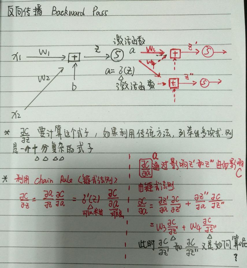
对于此处的
则此时有
此时我们注意到,要计算

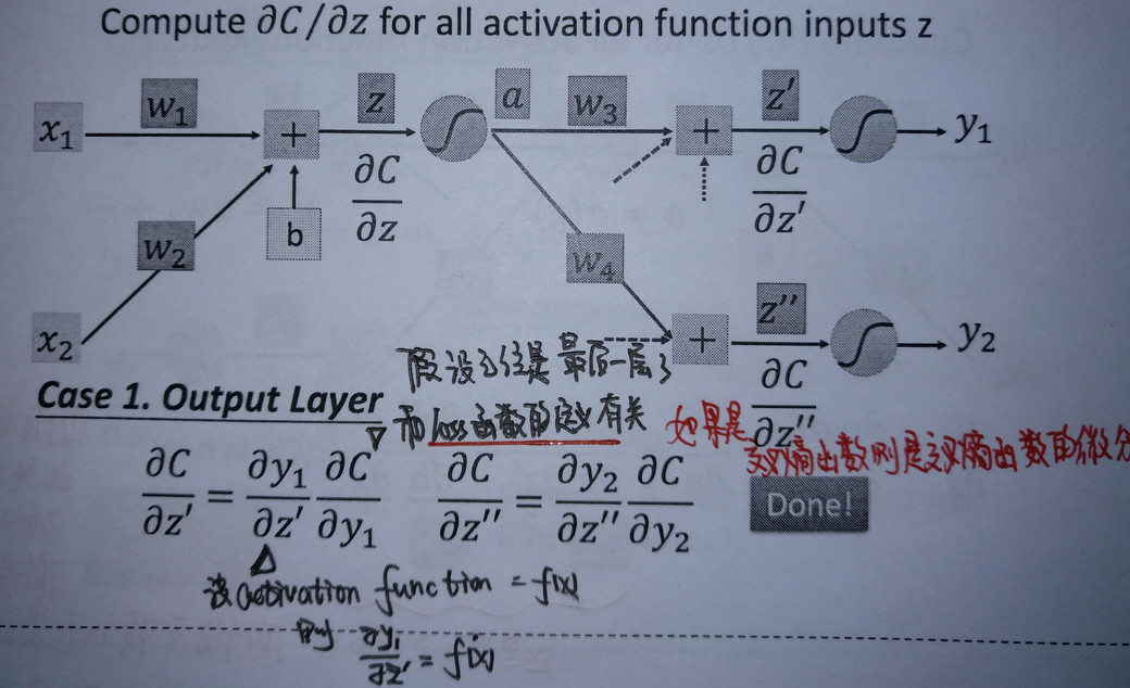
case1 output layer
- 假设此神经元已经是最后一层隐藏层神经元,其后连接的是输出层,有输出y1和y2.
case2 not output layer
- 假设此神经元不是最后一层隐藏层的神经元,即其后还有许多层的神经元.
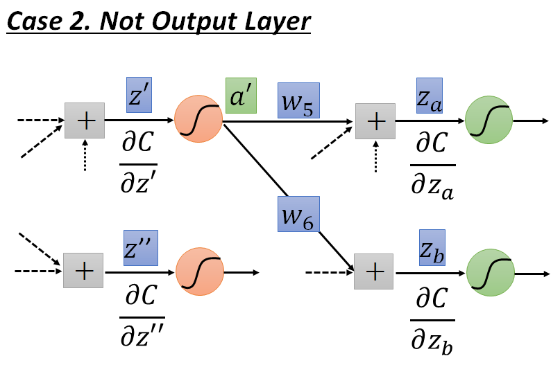
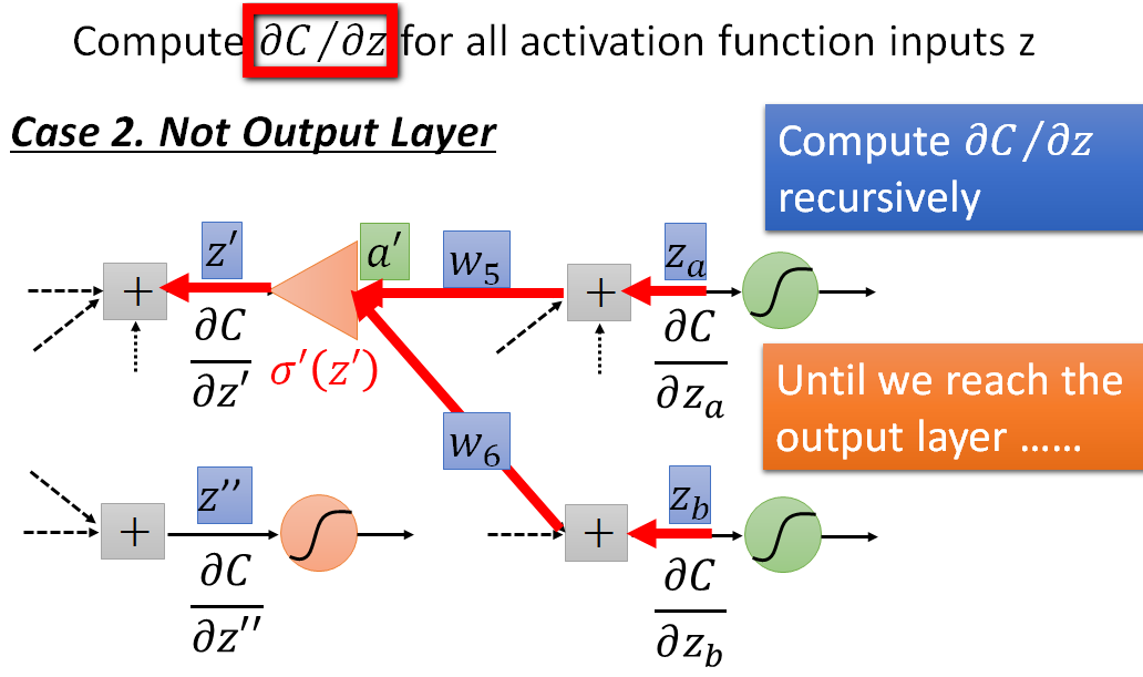
根据前面的模型我们知道,如果我们已知
∂C∂Za和∂C∂Zb那么我们可以求出∂C∂z′ ∂C∂Z′=(W5∗∂C∂Za+W6∗∂C∂Zb)∗σ′(Z′) 我们使用这个方法已知持续到最后一层隐藏层,我们可以按照最后一层为隐藏层的方法从后向前进行推导
summary
- BP算法可以理解为逆向的建立一个神经网络,这个神经网络的激励函数是
σ′(Zn) ,这需要通过神经网络的Forward pass前向传播才能得到. - 接下来我们可以通过最后一个隐层求得
∂C∂Z5和∂C∂z6 - 接下来和普通的神经网络一样对其进行运算求得结果
空说无凭,来看代码


import randomimport math## Shorthand:# "pd_" as a variable prefix means "partial derivative"# "d_" as a variable prefix means "derivative"# "_wrt_" is shorthand for "with respect to"# "w_ho" and "w_ih" are the index of weights from hidden to output layer neurons and input to hidden layer neurons respectively## Comment references:## [1] Wikipedia article on Backpropagation# http://en.wikipedia.org/wiki/Backpropagation#Finding_the_derivative_of_the_error# [2] Neural Networks for Machine Learning course on Coursera by Geoffrey Hinton# https://class.coursera.org/neuralnets-2012-001/lecture/39# [3] The Back Propagation Algorithm# https://www4.rgu.ac.uk/files/chapter3%20-%20bp.pdf# [4] The original location of the code# https://github.com/mattm/simple-neural-network/blob/master/neural-network.pyclass NeuralNetwork: # 神经网络类 LEARNING_RATE = 0.5 # 设置学习率为0.5 def __init__(self, num_inputs, num_hidden, num_outputs, hidden_layer_weights=None, hidden_layer_bias=None, output_layer_weights=None, output_layer_bias=None): # 初始化一个三层神经网络结构 self.num_inputs = num_inputs self.hidden_layer = NeuronLayer(num_hidden, hidden_layer_bias) self.output_layer = NeuronLayer(num_outputs, output_layer_bias) self.init_weights_from_inputs_to_hidden_layer_neurons(hidden_layer_weights) self.init_weights_from_hidden_layer_neurons_to_output_layer_neurons(output_layer_weights) def init_weights_from_inputs_to_hidden_layer_neurons(self, hidden_layer_weights): weight_num = 0 for h in range(len(self.hidden_layer.neurons)): # num_hidden,遍历隐藏层 for i in range(self.num_inputs): # 遍历输入层 if not hidden_layer_weights: # 如果hidden_layer_weights的值为空,则利用随机化函数对其进行赋值,否则利用hidden_layer_weights中的值对其进行更新 self.hidden_layer.neurons[h].weights.append(random.random()) else: self.hidden_layer.neurons[h].weights.append(hidden_layer_weights[weight_num]) weight_num += 1 def init_weights_from_hidden_layer_neurons_to_output_layer_neurons(self, output_layer_weights): weight_num = 0 for o in range(len(self.output_layer.neurons)): # num_outputs,遍历输出层 for h in range(len(self.hidden_layer.neurons)): # 遍历输出层 if not output_layer_weights: # 如果output_layer_weights的值为空,则利用随机化函数对其进行赋值,否则利用output_layer_weights中的值对其进行更新 self.output_layer.neurons[o].weights.append(random.random()) else: self.output_layer.neurons[o].weights.append(output_layer_weights[weight_num]) weight_num += 1 def inspect(self): # 输出神经网络信息 print('------') print('* Inputs: {}'.format(self.num_inputs)) print('------') print('Hidden Layer') self.hidden_layer.inspect() print('------') print('* Output Layer') self.output_layer.inspect() print('------') def feed_forward(self, inputs): # 返回输出层y值 hidden_layer_outputs = self.hidden_layer.feed_forward(inputs) return self.output_layer.feed_forward(hidden_layer_outputs) # Uses online learning, ie updating the weights after each training case # 使用在线学习方式,训练每个实例之后对权值进行更新 def train(self, training_inputs, training_outputs): self.feed_forward(training_inputs) # 反向传播 # 1. Output neuron deltas输出层deltas pd_errors_wrt_output_neuron_total_net_input = [0]*len(self.output_layer.neurons) for o in range(len(self.output_layer.neurons)): # 对于输出层∂E/∂zⱼ=∂E/∂a*∂a/∂z=cost'(target_output)*sigma'(z) pd_errors_wrt_output_neuron_total_net_input[o] = self.output_layer.neurons[ o].calculate_pd_error_wrt_total_net_input(training_outputs[o]) # 2. Hidden neuron deltas隐藏层deltas pd_errors_wrt_hidden_neuron_total_net_input = [0]*len(self.hidden_layer.neurons) for h in range(len(self.hidden_layer.neurons)): # We need to calculate the derivative of the error with respect to the output of each hidden layer neuron # 我们需要计算误差对每个隐藏层神经元的输出的导数,由于不是输出层所以dE/dyⱼ需要根据下一层反向进行计算,即根据输出层的函数进行计算 # dE/dyⱼ = Σ ∂E/∂zⱼ * ∂z/∂yⱼ = Σ ∂E/∂zⱼ * wᵢⱼ d_error_wrt_hidden_neuron_output = 0 for o in range(len(self.output_layer.neurons)): d_error_wrt_hidden_neuron_output += pd_errors_wrt_output_neuron_total_net_input[o]* \ self.output_layer.neurons[o].weights[h] # ∂E/∂zⱼ = dE/dyⱼ * ∂zⱼ/∂ pd_errors_wrt_hidden_neuron_total_net_input[h] = d_error_wrt_hidden_neuron_output*self.hidden_layer.neurons[ h].calculate_pd_total_net_input_wrt_input() # 3. Update output neuron weights 更新输出层权重 for o in range(len(self.output_layer.neurons)): for w_ho in range(len(self.output_layer.neurons[o].weights)): # 注意:输出层权重是隐藏层神经元与输出层神经元连接的权重 # ∂Eⱼ/∂wᵢⱼ = ∂E/∂zⱼ * ∂zⱼ/∂wᵢⱼ pd_error_wrt_weight = pd_errors_wrt_output_neuron_total_net_input[o]*self.output_layer.neurons[ o].calculate_pd_total_net_input_wrt_weight(w_ho) # Δw = α * ∂Eⱼ/∂wᵢ self.output_layer.neurons[o].weights[w_ho] -= self.LEARNING_RATE*pd_error_wrt_weight # 4. Update hidden neuron weights 更新隐藏层权重 for h in range(len(self.hidden_layer.neurons)): for w_ih in range(len(self.hidden_layer.neurons[h].weights)): # 注意:隐藏层权重是输入层神经元与隐藏层神经元连接的权重 # ∂Eⱼ/∂wᵢ = ∂E/∂zⱼ * ∂zⱼ/∂wᵢ pd_error_wrt_weight = pd_errors_wrt_hidden_neuron_total_net_input[h]*self.hidden_layer.neurons[ h].calculate_pd_total_net_input_wrt_weight(w_ih) # Δw = α * ∂Eⱼ/∂wᵢ self.hidden_layer.neurons[h].weights[w_ih] -= self.LEARNING_RATE*pd_error_wrt_weight def calculate_total_error(self, training_sets): # 使用平方差计算训练集误差 total_error = 0 for t in range(len(training_sets)): training_inputs, training_outputs = training_sets[t] self.feed_forward(training_inputs) for o in range(len(training_outputs)): total_error += self.output_layer.neurons[o].calculate_error(training_outputs[o]) return total_errorclass NeuronLayer: # 神经层类 def __init__(self, num_neurons, bias): # Every neuron in a layer shares the same bias 一层中的所有神经元共享一个bias self.bias = bias if bias else random.random() random.random() # 生成0和1之间的随机浮点数float,它其实是一个隐藏的random.Random类的实例的random方法。 # random.random()和random.Random().random()作用是一样的。 self.neurons = [] for i in range(num_neurons): self.neurons.append(Neuron(self.bias)) # 在神经层的初始化函数中对每一层的bias赋值,利用神经元的init函数对神经元的bias赋值 def inspect(self): # print该层神经元的信息 print('Neurons:', len(self.neurons)) for n in range(len(self.neurons)): print(' Neuron', n) for w in range(len(self.neurons[n].weights)): print(' Weight:', self.neurons[n].weights[w]) print(' Bias:', self.bias) def feed_forward(self, inputs): # 前向传播过程outputs中存储的是该层每个神经元的y/a的值(经过神经元激活函数的值有时被称为y有时被称为a) outputs = [] for neuron in self.neurons: outputs.append(neuron.calculate_output(inputs)) return outputs def get_outputs(self): outputs = [] for neuron in self.neurons: outputs.append(neuron.output) return outputsclass Neuron: # 神经元类 def __init__(self, bias): self.bias = bias self.weights = [] def calculate_output(self, inputs): self.inputs = inputs self.output = self.squash(self.calculate_total_net_input()) # output即为输入即为y(a)意为从激活函数中的到的值 return self.output def calculate_total_net_input(self): # 此处计算的为激活函数的输入值即z=W(n)x+b total = 0 for i in range(len(self.inputs)): total += self.inputs[i]*self.weights[i] return total + self.bias # Apply the logistic function to squash the output of the neuron # 使用sigmoid函数为激励函数,一下是sigmoid函数的定义 # The result is sometimes referred to as 'net' [2] or 'net' [1] def squash(self, total_net_input): return 1/(1 + math.exp(-total_net_input)) # Determine how much the neuron's total input has to change to move closer to the expected output # 确定神经元的总输入需要改变多少,以接近预期的输出 # Now that we have the partial derivative of the error(Cost function) with respect to the output (∂E/∂yⱼ) # 我们可以根据cost function对y(a)神经元激活函数输出值的偏导数和激活函数输出值y(a)对激活函数输入值z=wx+b的偏导数计算delta(δ). # the derivative of the output with respect to the total net input (dyⱼ/dzⱼ) we can calculate # the partial derivative of the error with respect to the total net input. # This value is also known as the delta (δ) [1] # δ = ∂E/∂zⱼ = ∂E/∂yⱼ * dyⱼ/dzⱼ 关键key # def calculate_pd_error_wrt_total_net_input(self, target_output): return self.calculate_pd_error_wrt_output(target_output)*self.calculate_pd_total_net_input_wrt_input() # The error for each neuron is calculated by the Mean Square Error method: # 每个神经元的误差由平均平方误差法计算 def calculate_error(self, target_output): return 0.5*(target_output - self.output) ** 2 # The partial derivate of the error with respect to actual output then is calculated by: # 对实际输出的误差的偏导是通过计算得到的--即self.output(y也常常用a表示经过激活函数后的值) # = 2 * 0.5 * (target output - actual output) ^ (2 - 1) * -1 # = -(target output - actual output)BP算法最后隐层求cost function 对a求导 # # The Wikipedia article on backpropagation [1] simplifies to the following, but most other learning material does not [2] # 维基百科关于反向传播[1]的文章简化了以下内容,但大多数其他学习材料并没有简化这个过程[2] # = actual output - target output # # Note that the actual output of the output neuron is often written as yⱼ and target output as tⱼ so: # = ∂E/∂yⱼ = -(tⱼ - yⱼ) # 注意我们一般将输出层神经元的输出为yⱼ,而目标标签(正确答案)表示为tⱼ. def calculate_pd_error_wrt_output(self, target_output): return -(target_output - self.output) # The total net input into the neuron is squashed using logistic function to calculate the neuron's output: # yⱼ = φ = 1 / (1 + e^(-zⱼ)) 注意我们对于神经元使用的激活函数都是logistic函数 # Note that where ⱼ represents the output of the neurons in whatever layer we're looking at and ᵢ represents the layer below it # 注意我们用j表示我们正在看的这层神经元的输出,我们用i表示这层的后一层的神经元. # The derivative (not partial derivative since there is only one variable) of the output then is: # dyⱼ/dzⱼ = yⱼ * (1 - yⱼ)这是sigmoid函数的导数表现形式. def calculate_pd_total_net_input_wrt_input(self): return self.output*(1 - self.output) # The total net input is the weighted sum of all the inputs to the neuron and their respective weights: # 激活函数的输入是所有输入的加权权重的总和 # = zⱼ = netⱼ = x₁w₁ + x₂w₂ ... # The partial derivative of the total net input with respective to a given weight (with everything else held constant) then is: # 总的净输入与给定的权重的偏导数(其他所有的项都保持不变) # = ∂zⱼ/∂wᵢ = some constant + 1 * xᵢw₁^(1-0) + some constant ... = xᵢ def calculate_pd_total_net_input_wrt_weight(self, index): return self.inputs[index]# Blog post example:nn = NeuralNetwork(2, 2, 2, hidden_layer_weights=[0.15, 0.2, 0.25, 0.3], hidden_layer_bias=0.35, output_layer_weights=[0.4, 0.45, 0.5, 0.55], output_layer_bias=0.6)for i in range(10000): nn.train([0.05, 0.1], [0.01, 0.99]) print(i, round(nn.calculate_total_error([[[0.05, 0.1], [0.01, 0.99]]]), 9)) # 截断处理只保留小数点后9位# XOR example:# training_sets = [# [[0, 0], [0]],# [[0, 1], [1]],# [[1, 0], [1]],# [[1, 1], [0]]# ]# nn = NeuralNetwork(len(training_sets[0][0]), 5, len(training_sets[0][1]))# for i in range(10000):# training_inputs, training_outputs = random.choice(training_sets)# nn.train(training_inputs, training_outputs)# print(i, nn.calculate_total_error(training_sets))阅读全文
0 0
- BP算法从原理到python实现
- PageRank算法--从原理到实现
- HITS算法--从原理到实现
- HITS算法--从原理到实现
- PageRank算法--从原理到实现
- PageRank算法--从原理到实现
- HITS算法--从原理到实现
- PageRank算法--从原理到实现
- PageRank算法--从原理到实现
- BP神经网络原理推到&代码实现
- BP神经网络原理及实现算法
- 机器学习算法-K最近邻从原理到实现(Python)
- 干货|从决策树到随机森林:树型算法的实现原理与Python 示例
- 神经网络中 BP 算法的原理与 PYTHON 实现源码解析
- 神经网络中 BP 算法的原理与 Python 实现源码解析
- Python 实现 周志华 《机器学习》 BP算法
- bp算法python实现(bpnn.py)
- BP算法推导(python实现)
- JavaScript代码规范
- 迅雷5.8稳定版工具
- [SCOI2005]繁忙的都市
- 富文本编辑器三种不同图片上传功能
- 习题为例学习K近邻简单实现
- BP算法从原理到python实现
- 遍历与复制数组
- 我的第一个Python+Appium脚本之APP登录脚本
- 腾讯云root用户
- Android自定义View之使用Path绘制手势轨迹和水波效果
- net-snmp开发过程整理-简介
- LeetCode160. Intersection of Two Linked Lists
- 理解泰勒公式·漫画
- Android 通用流行框架大全