The Predator-Prey Equation in Matlab

转载自：http://www-users.math.umd.edu/~jmr/246/predprey.html

 

 

 

The Predator-Prey Equation

Contents

• Original Lotka-Volterra Model
• Critical points:
• Phase Plot
• Plot of Populations vs. Time
• Modified Model with "Limits to Growth" for Prey (in Absence of Predators)
• Critical points:
• Plot of Populations vs. Time

Original Lotka-Volterra Model

We assume we have two species, herbivores with population x, and predators with propulation y. We assume that x grows exponentially in the absence of predators, and that y decays exponentially in the absence of prey. Consider, say, the system

Critical points:

syms x yvars = [x, y];eqs = [x*(1-y/2), y*(-1+x/2)];[xc, yc] = solve(eqs(1), eqs(2));[xc, yc]A = jacobian(eqs, vars);disp('Matrix of linearized system:')subs(A, vars, [xc(1), yc(1)])disp('eigenvalues:')eig(ans)disp('Matrix of linearized system:')subs(A, vars, [xc(2), yc(2)])disp('eigenvalues:')eig(double(ans))

 ans = [ 0, 0][ 2, 2]  Matrix of linearized system: ans = [  1,  0][  0, -1]  eigenvalues: ans =   1 -1  Matrix of linearized system: ans = [  0, -1][  1,  0]  eigenvalues:ans =        0 + 1.0000i        0 - 1.0000i

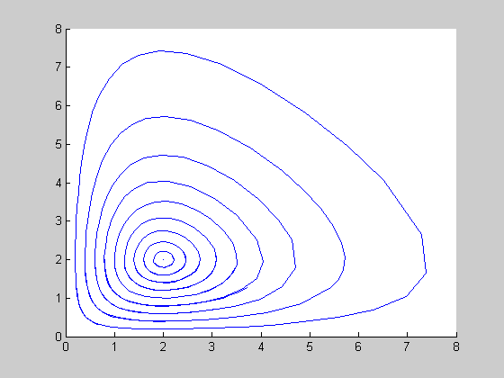
Thus we have a center at (2, 2) and a saddle point at (0, 0), at least for the linearized system. This suggests the possibility of periodic orbits centered around (2, 2).

Phase Plot

rhs1 = @(t, x) ...    [x(1)*(1-.5*x(2)); x(2)*(-1+.5*x(1))];options = odeset('RelTol', 1e-6);figure, hold onfor x0 = 0:.2:2    [t, x] = ode45(rhs1, [0, 10], [x0;2]);    plot(x(:,1), x(:,2))end, hold off

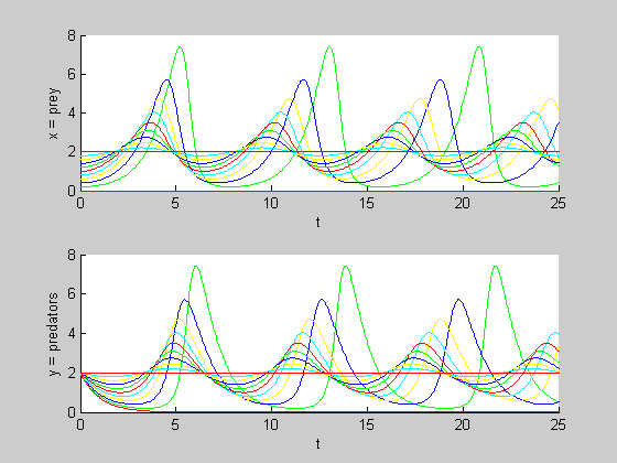
Plot of Populations vs. Time

We color-code the plots so you can see which ones go together.

colors = 'rgbyc';figure, hold onfor x0 = 0:10    [t, x] = ode45(rhs1, [0, 25], [x0/5; 2], options);    subplot(2, 1, 1), hold on    plot(t, x(:,1), colors(mod(x0,5)+1))    subplot(2, 1, 2), hold on    plot(t, x(:, 2), colors(mod(x0,5)+1))    hold onendsubplot(2, 1, 1)xlabel tylabel 'x = prey'subplot(2, 1, 2)xlabel tylabel 'y = predators'hold off

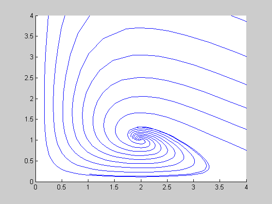
Modified Model with "Limits to Growth" for Prey (in Absence of Predators)

In the original equation, the population of prey increases indefinitely in the absence of predators. This is unrealistic, since they will eventually run out of food, so let's add another term limiting growth and change the system to

Critical points:

syms x yvars = [x, y];eqs = [x*(1-y/2-x/4), y*(-1+x/2)];[xc, yc] = solve(eqs(1), eqs(2));[xc, yc]A = jacobian(eqs, vars);disp('Matrix of linearized system:')subs(A, vars, [xc(1), yc(1)])disp('eigenvalues:')eig(ans)disp('Matrix of linearized system:')subs(A, vars, [xc(2), yc(2)])disp('eigenvalues:')eig(ans)disp('Matrix of linearized system:')subs(A, vars, [xc(3), yc(3)])disp('eigenvalues:')eig(double(ans))

 ans = [ 0, 0][ 4, 0][ 2, 1]  Matrix of linearized system: ans = [  1,  0][  0, -1]  eigenvalues: ans =   1 -1  Matrix of linearized system: ans = [ -1, -2][  0,  1]  eigenvalues: ans =  -1  1  Matrix of linearized system: ans = [ -1/2,   -1][  1/2,    0]  eigenvalues:ans =  -0.2500 + 0.6614i  -0.2500 - 0.6614i

Thus we have saddles at (0, 0), (4, 0) and a stable spiral point at (2, 1).

rhs2 = @(t, x) ...    [x(1)*(1-.5*x(2)-0.25*x(1)); x(2)*(-1+.5*x(1))];figure, hold onfor x0 = 0:.2:2    [t, x] = ode45(rhs2, [0, 10], [x0;1]);    plot(x(:,1), x(:,2))endfor x0 = 0:.2:2    [t, x] = ode45(rhs2, [0, -10], [x0;1]);    plot(x(:,1), x(:,2))endaxis([0, 4, 0, 4]), hold off

Warning: Failure at t=-3.380660e+000.  Unable to meet integration tolerances without reducing the step size below the smallest value allowed (7.105427e-015) at time t.Warning: Failure at t=-3.535072e+000.  Unable to meet integration tolerances without reducing the step size below the smallest value allowed (7.105427e-015) at time t.Warning: Failure at t=-3.735844e+000.  Unable to meet integration tolerances without reducing the step size below the smallest value allowed (7.105427e-015) at time t.Warning: Failure at t=-3.984664e+000.  Unable to meet integration tolerances without reducing the step size below the smallest value allowed (7.105427e-015) at time t.Warning: Failure at t=-4.299922e+000.  Unable to meet integration tolerances without reducing the step size below the smallest value allowed (1.421085e-014) at time t.Warning: Failure at t=-4.719481e+000.  Unable to meet integration tolerances without reducing the step size below the smallest value allowed (1.421085e-014) at time t.Warning: Failure at t=-5.332082e+000.  Unable to meet integration tolerances without reducing the step size below the smallest value allowed (1.421085e-014) at time t.Warning: Failure at t=-6.437607e+000.  Unable to meet integration tolerances without reducing the step size below the smallest value allowed (1.421085e-014) at time t.

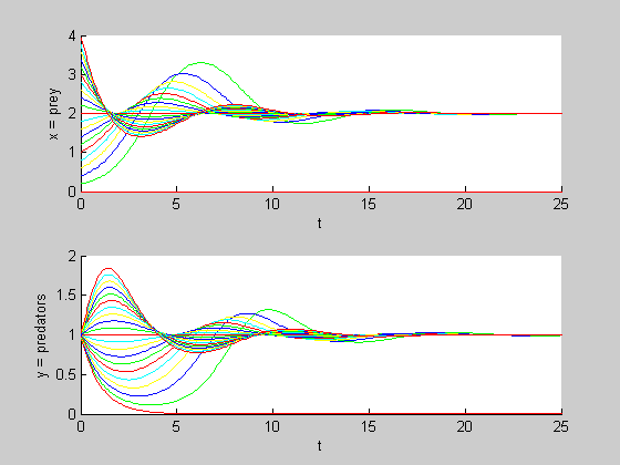
Plot of Populations vs. Time

figure, hold onfor x0 = 0:20    [t, x] = ode45(rhs2, [0, 25], [x0/5; 1], options);    subplot(2, 1, 1), hold on    plot(t, x(:,1), colors(mod(x0,5)+1))    subplot(2, 1, 2), hold on    plot(t, x(:, 2), colors(mod(x0,5)+1))    hold onendsubplot(2, 1, 1)xlabel tylabel 'x = prey'subplot(2, 1, 2)xlabel tylabel 'y = predators'hold off

Published with MATLAB® 7.0