OpenCV Tutorial 6 - Chapter 7

 Author: Noah Kuntz (2009)
Contact: [e-mail]

Keywords: OpenCV, computer vision, image processing, histograms

My Vision Tutorials Index

This tutorial assumes the reader:
(1) Has a basic knowledge of Visual C++
(2) Has some familiarity with computer vision concepts
(3) Has read the previous tutorials in this series

The rest of the tutorial is presented as follows:

• Step 1: Histograms and Back Projection
• Step 2: Template Matching
• Final Words

Important Note!

More information on the topics of these tutorials can be found in this book:Learning OpenCV: Computer Vision with the OpenCV Library

Step 1: Histograms and Back Projection（直方图和反投影）

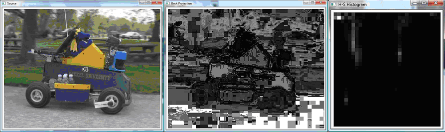
Original Image, Back Projection, and Histogram

(原始图像，背投，和直方图)

Histograms are one of the classic methods to analyze images（直方图是分析图像的经典方法之一）. A Histogram classifies aspects of an image into  bins to determine the correlation between images, or a feature in an image（直方图把图像方面划分成箱，以确定图像之间的相关性，或者图像的功能）. OpenCV provides theCvHistogram structure, created with cvCreateHist(int dims, int* sizes, int type, float** ranges = NULL, int uniform = 1) （OpenCV中提供了CvHistogram结构，用cvCreateHist(int dims, int* sizes, int type, float** ranges = NULL, int uniform = 1来创建）.Consult the book for more details of the histogram data structure（咨询本书获得更多直方图数据结构的详细资料）. Histograms bins are accessed in a similiar way to normal matrices, for example withcvGetHistValue_2D(CvHistogram* hist, int idx0, idx1)（直方图箱的访问方式类似于访问正常的矩阵，例如cvGetHistValue_2D(CvHistogram* hist, int idx0, idx1）. The following example computes a histogram for the intensity of an image based on the HSV colorspace（下面的示例是在HSV色彩空间的基础上计算一幅图像的亮度直方图）. The histogram is also normalized, andcvCalcBackProject is used to map the histogram results back on to the image to better illustrate the results（直方图总是被正常化的，cvCalcBackProject用于以更好的说明结果把直方图结果映射传回到图像上）. Here is the code（以下是代码）:

---

int _tmain(int argc, _TCHAR* argv[])

{

        // Set up images

        IplImage* img = cvLoadImage("MGC.jpg");

        IplImage* back_img = cvCreateImage( cvGetSize( img ), IPL_DEPTH_8U, 1 );

 

        // Compute HSV image and separate into colors

        IplImage* hsv = cvCreateImage( cvGetSize(img), IPL_DEPTH_8U, 3 );

        cvCvtColor( img, hsv, CV_BGR2HSV );

 

        IplImage* h_plane = cvCreateImage( cvGetSize( img ), 8, 1 );

        IplImage* s_plane = cvCreateImage( cvGetSize( img ), 8, 1 );

        IplImage* v_plane = cvCreateImage( cvGetSize( img ), 8, 1 );

        IplImage* planes[] = { h_plane, s_plane };

        cvCvtPixToPlane( hsv, h_plane, s_plane, v_plane, 0 );

 

        // Build and fill the histogram

        int h_bins = 30, s_bins = 32;

        CvHistogram* hist;

        {

               int hist_size[] = { h_bins, s_bins };

               float h_ranges[] = { 0, 180 };

               float s_ranges[] = { 0, 255 };

               float* ranges[] = { h_ranges, s_ranges };

               hist = cvCreateHist( 2, hist_size, CV_HIST_ARRAY, ranges, 1 );

        }

        cvCalcHist( planes, hist, 0, 0 ); // Compute histogram

        cvNormalizeHist( hist, 20*255 ); // Normalize it

 

        cvCalcBackProject( planes, back_img, hist );// Calculate back projection

        cvNormalizeHist( hist, 1.0 ); // Normalize it

 

       

       

        // Create an image to visualize the histogram

        int scale = 10;

        IplImage* hist_img = cvCreateImage( cvSize( h_bins * scale, s_bins * scale ), 8, 3 );

        cvZero ( hist_img );

 

        // populate the visualization

        float max_value = 0;

        cvGetMinMaxHistValue( hist, 0, &max_value, 0, 0 );

 

        for( int h = 0; h < h_bins; h++ ){

               for( int s = 0; s < s_bins; s++ ){

                       float bin_val = cvQueryHistValue_2D( hist, h, s );

                       int intensity = cvRound( bin_val * 255 / max_value );

                       cvRectangle( hist_img, cvPoint( h*scale, s*scale ),

                                              cvPoint( (h+1)*scale - 1, (s+1)*scale - 1 ),

                                              CV_RGB( intensity, intensity, intensity ),

                                              CV_FILLED );

               }

        }

 

        // Show original

        cvNamedWindow( "Source", 1) ;

        cvShowImage( "Source", img );

 

        // Show back projection

        cvNamedWindow( "Back Projection", 1) ;

        cvShowImage( "Back Projection", back_img );

 

        // Show histogram equalized

        cvNamedWindow( "H-S Histogram", 1) ;

        cvShowImage( "H-S Histogram", hist_img );

 

        cvWaitKey(0);

 

        cvReleaseImage( &img );

        cvReleaseImage( &back_img );

        cvReleaseImage( &hist_img );

 

        return 0;

}

 

---

Step 2: Template Matching（模板匹配）

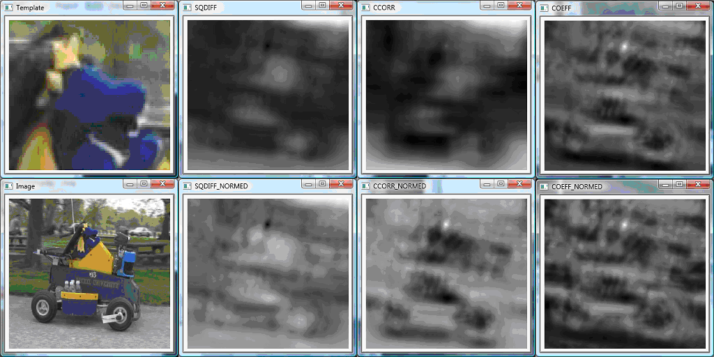
Histogram Template Matching（直方图模板匹配）

Another powerful operation with a histogram is template matching（另一个是一个强大的直方图操作是模板匹配）. Here a template image is compared with a larger image to find the area most similiar to the template in the larger image（这里是把一个模板图像与一幅较大的图像进行比较，来找出这个较大图像中与模板最相似的区域）. The function cvMatchTemplate( const CvArr* image, const CvArr* templ, CvArr* result, int method ) is used to do the matching（函数cvMatchTemplate( const CvArr* image, const CvArr* templ, CvArr* result, int method )是用来做匹配）. The last input here chooses is the method of template matching（这里选择的最后一个输入是模板匹配方法）. We use all six methods, starting with square difference matching, which simply takes the squared difference between the template and image（我们使用的所有六种方法，开始与平方差匹配，这只是简单地采用模板和图像之间的平方差）. A good match is 0 and bad matches are large values（一个好的匹配的误差是0，差的匹配是很大的值）. Then there is correlation matching which multiplies the template against the image, so a large value is a good match and a very bad match is 0  .（其次是相关匹配，它乘以模板对图像，因此一个较大的值是一个很好的匹配和一个非常坏的匹配是0）. The last general type of matching is correlation coefficient matching, which matches the mean of the image relative to the mean of template, with a good match being 1, no match being 0, and a mismatch being as low as -1（最后一个普通的匹配类型是相关系数匹配，它匹配图像的平均相对于模板的平均，一个好的匹配为1，不匹配为0，并且错误匹配低至-1）. The normalized versions of these are also tested, and generally provide more visually clear results这些归一的版本也是被测试的，并全面地提供了更直观明显的成效）. Here is the code（以下是代码）:

---

int _tmain(int argc, _TCHAR* argv[])

{

        IplImage *src, *templ, *ftmp[6]; // ftmp will hold results

        int i;

 

        // Read in the source image to be searched

        src = cvLoadImage("MGC.jpg");

 

        // Read in the template to be used for matching:

        templ = cvLoadImage("template.jpg");

 

        // Allocate Output Images:

        int iwidth = src->width - templ->width + 1;

        int iheight = src->height - templ->height + 1;

        for(i = 0; i < 6; ++i){

               ftmp[i]= cvCreateImage( cvSize( iwidth, iheight ), 32, 1 );

        }

 

        // Do the matching of the template with the image

        for( i = 0; i < 6; ++i ){

               cvMatchTemplate( src, templ, ftmp[i], i );

               cvNormalize( ftmp[i], ftmp[i], 1, 0, CV_MINMAX );

        }

 

        // DISPLAY

        cvNamedWindow( "Template", 0 );

        cvShowImage( "Template", templ );

        cvNamedWindow( "Image", 0 );

        cvShowImage( "Image", src );

        cvNamedWindow( "SQDIFF", 0 );

        cvShowImage( "SQDIFF", ftmp[0] );

        cvNamedWindow( "SQDIFF_NORMED", 0 );

        cvShowImage( "SQDIFF_NORMED", ftmp[1] );

        cvNamedWindow( "CCORR", 0 );

        cvShowImage( "CCORR", ftmp[2] );

        cvNamedWindow( "CCORR_NORMED", 0 );

        cvShowImage( "CCORR_NORMED", ftmp[3] );

        cvNamedWindow( "COEFF", 0 );

        cvShowImage( "COEFF", ftmp[4] );

        cvNamedWindow( "COEFF_NORMED", 0 );

        cvShowImage( "COEFF_NORMED", ftmp[5] );

 

        cvWaitKey(0);

        return 0;

}

---

 

Final Words（结束语）

This tutorial's objective was to show how to use some basic histogram functions（本教程的目标是展示如何使用一些基本的直方图功能）.

Click here to email me.
Click here to return to my Tutorials page.