jvm performance tunning

1. use jmap and jhat 

    jmap-- Memory Map prints shared object memory maps or heap memory details of a given process or core file or a remote debug server

   

jmap [ option ] pidjmap [ option ] executable corejmap [ option ] [server-id@]remote-hostname-or-IP

    Notice: pid must be process of java, we can use `jps` command to find the pid.

显示java进程内存使用的相关信息

• jmap pid #打印内存使用的摘要信息
• jmap –heap pid #java heap信息
• jmap -histo:live pid #统计对象count ，live表示在使用
• jmap -histo pid >mem.txt #打印比较简单的各个有多少个对象占了多少内存的信息，一般重定向的文件
• jmap -dump:format=b,file=mem.dat pid #将内存使用的详细情况输出到mem.dat 文件

And JDK jvisualvm.exe can monitor the local and remote application and performance.  可以用它解决内存溢出问题，eg, 如何PermGen, 从monitor中的视图中看到PermGen在程序运行一段时间后超出了指定的范围，根据图中的图示可以看到是class的大量load原因还是其他的原因，为了使应用稳定，我们需要找PermGen的稳定范围。例如通过监测发现145m是它的稳定范围，那我们就得到了稳定的新参数。内存溢出问题也就解决了。

Unfinished.

------------------------------

The following part is from internet

---------------------------------------------

1.jps                 
.:与unix上的ps类似，用来显示本地的java进程，可以查看本地运行着几个java程序，并显示他们的进程号。                    

2.jstat                 
.:一个极强的监视VM内存工具。可以用来监视VM内存内的各种堆和非堆的大小及其内存使用量。                    
            
3.jmap                 
.:打印出某个java进程（使用pid）内存内的，所有‘对象’的情况（如：产生那些对象，及其数量）。                    
4.jconsole                
.:一个java GUI监视工具，可以以图表化的形式显示各种数据。并可通过远程连接监视远程的服务器VM。    

二、 使用介绍： 
    
    1、jps ：我想很多人都是用过unix系统里的ps命令，这个命令主要是用来显示当前系统的进程情况，有哪些进程，及其 id。 jps 也是一样，它的作用是显示当前系统的java(jvm 进程)进程情况，及其id号。我们可以通过它来查看我们到底启动了几个java进程（因为每一个java程序都会独占一个java虚拟机实例），和他们的进程号（为下面几个程序做准备），并可通过opt来查看这些进程的详细启动参数。 
    使用方法：在当前命令行下打 jps(需要JAVA_HOME，没有的话，到改程序的目录下打) 。

可惜没有linux下的ps好用，名称不好用。但是在第四个工具jconsole的界面里面会有具体JAR包的名称。

/data/jdk1.6.0_06/bin/jps    
6360 Resin 
6322 WatchdogManager 
2466 Jps

      
    2、jstat ：对VM内存使用量进行监控。 
    jstat工具特别强大，有众多的可选项，详细查看堆内各个部分的使用量，以及加载类的数量。使用时，需加上查看进程的进程id，和所选参数。以下详细介绍各个参数的意义。 
    jstat -class pid:显示加载class的数量，及所占空间等信息。 
    jstat -compiler pid:显示VM实时编译的数量等信息。 
    jstat -gc pid:可以显示gc的信息，查看gc的次数，及时间。其中最后五项，分别是young gc的次数，young gc的时间，full gc的次数，full gc的时间，gc的总时间。 
    jstat -gccapacity:可以显示，VM内存中三代（young,old,perm）对象的使用和占用大小，如：PGCMN显示的是最小perm的内存使用量，PGCMX显示的是perm的内存最大使用量，PGC是当前新生成的perm内存占用量，PC是但前perm内存占用量。其他的可以根据这个类推， OC是old内纯的占用量。 
    jstat -gcnew pid:new对象的信息。 
    jstat -gcnewcapacity pid:new对象的信息及其占用量。 
    jstat -gcold pid:old对象的信息。 
    jstat -gcoldcapacity pid:old对象的信息及其占用量。 
    jstat -gcpermcapacity pid: perm对象的信息及其占用量。 
    jstat -util pid:统计gc信息统计。 
    jstat -printcompilation pid:当前VM执行的信息。 
    除了以上一个参数外，还可以同时加上 两个数字，如：jstat -printcompilation 3024 250 6是每250毫秒打印一次，一共打印6次，还可以加上-h3每三行显示一下标题。 
    
   3、jmap 是一个可以输出所有内存中对象的工具，甚至可以将VM 中的heap，以二进制输出成文本。使用方法 jmap -histo pid。如果连用 SHELL jmap -histo pid>a.log可以将其保存到文本中去（windows下也可以使用），在一段时间后，使用文本对比工具，可以对比出GC回收了哪些对象。jmap -dump:format=b,file=f1 3024可以将3024进程的内存heap输出出来到f1文件里。 
    
    4、jconsole 是一个用java写的GUI程序，用来监控VM，并可监控远程的VM，非常易用，而且功能非常强。由于是GUI程序，这里就不详细介绍了，不会的地方可以参考ＳＵＮ的官方文档。 
    使用方法：命令行里打 jconsole，选则进程就可以了。 
    
    友好提示：windows查看进程号，由于任务管理器默认的情况下是不显示进程id号的，所以可以通过如下方法加上。ctrl+alt+del打开任务管理器，选择‘进程’选项卡，点‘查看’->''选择列''->加上''PID''，就可以了。当然还有其他很好的选项。

实例：

jmap -histo:live $pid
jmap -histo $pid 
jstack -l $pid

5. jinfo

JVM监控工具之jinfo（linux下特有）

观察运行中的java程序的运行环境参数：参数包括JavaSystem属性和JVM命令行参数

jinfo <option> <pid>

三、参考资料：

    article:http://elf8848.javaeye.com/blog/442806

    jps:http://java.sun.com/j2se/1.5.0/docs/tooldocs/share/jps.html

    jstat:http://java.sun.com/j2se/1.5.0/docs/tooldocs/share/jstat.html

    jmap:http://java.sun.com/j2se/1.5.0/docs/tooldocs/share/jmap.html

    jconsole:http://java.sun.com/j2se/1.5.0/docs/guide/management/jconsole.html 

------------------------------------------------------

white paper about tunning from oracle official site

2   Best Practices

There are many best practices for getting the optimal performance with your Java application. Here are some very basic practices that can make a significant difference in performance before you begin tuning. 

2.1   Use the most recent Java™ release

Each major release of Java™ introduces new features, bug fixes and performance enhancements. Before you begin tuning or consider application level changes to take advantage of new language features it is still worthwhile to upgrade to the latest major Java™ release. For information on why upgrading to Java SE 5.0 (Tiger) is important please see the references in the Pointers section. 

Understandably this is not always possible as certain applications, especially third party ISV applications may not yet provide support for the latest release of Java™. In that case use the most recent update release which is supported for your application (and please encourage your ISV to support the latest Java™ version!). 

2.2   Get the latest Java™ update release

For each major Java™ release "train" (e.g. J2SE 1.3.1, J2SE 1.4.2, J2SE 5.0) Sun publishes update releases on a regular basis. For example the most recent update release of J2SE 5.0 is update 6 or Java SE 1.5.0_06. 

Update releases often include bug fixes and performance improvements. By deploying the most recent update release for Java™ you will benefit from the latest and greatest performance improvements. 

2.3   Insure your operating system patches are up-to-date

Even though Java is cross platform it does rely on the underlying operating system and therefore it is important that the OS basis for the Java™ Platform is as up-to-date as possible. 

In the case of Solaris there is a set of patches that are recommended when deploying Java applications. To get these Solaris patches for Java please see the links under the section Solaris OS Patches on the Java™ download page. 

2.4   Eliminate variability

Be aware that various system activities and the operations of other applications running on your system can introduce significant variance into the measurements of any application's performance, including Java applications. The activities of the OS and other applications may introduce CPU, Memory, disk or network resource contention that may interfere with your measurements. 

Before you begin to measure Java performance try to assess application behavior that may discolor your performance results (e.g. accessing the Internet for updates, reading files from the users home directory, etc.). By simplifying application behavior as much as possible and by changing only one variable at a time (i.e. operating system tunable parameter, Java command line option, application argument, etc.) your performance investigation can track the impact of each change independently. 

3   Making Decisions from Data

It is really tempting to run an application once before and once after a change and draw some conclusion about the impact of that change. Sometimes the application runs for a long time. Sometimes launching the application may be complex and dependent on multiple external services. But can you legitimately make a decision from this test? It's really impossible to know if you can safely draw a conclusion from the data unless you measure the power of the data quantitatively. Applying the scientific method is important when designing any set of experiments. Rigor is especially necessary when measuring Java application performance because the behavior of Java™ HotSpot™ virtual machine adapts and reacts to the specific machine and specific application it is running. And subtle changes in timing due to other system activity can result in measurable differences in performance and which are unrelated to the comparisons being made. 

3.1   Beware of Microbenchmarks!

One of the advantages of Java is that it dynamically optimizes for data at runtime. More and more we are finding cases where Java performance meets or exceeds the performance of similar statically compiled programs. However this adaptability of the JVM makes it hard to measure small snippets of Java functionality. 

One of the reasons that it's challenging to measure Java performance is that it changes over time. At startup, the JVM typically spends some time "warming up". Depending on the JVM implementation, it may spend some time in interpreted mode while it is profiled to find the 'hot' methods. When a method gets sufficiently hot, it may be compiled and optimized into native code. 

Indeed some of these optimizations may unroll loops, hoist variables outside of loops or even eliminate "dead code" altogether. So how should you handle this? Should you factor in the differences in machine speed by timing a few iterations of loop and then run a number of iterations that will give you similar total run time on each platform? If you do that what is likely to happen is your timing loop will estimate loop time while running in interpreted mode. Then when running the test the loop will get optimized and run much more quickly. So quickly, in fact, that your total run time might be so short that you are not measuring the inner loop at all but just the infrastructure for warming up the application. 

For certain applications garbage collection can complicate writing benchmarks. It is important to note, however, that for a given set of tuning parameters that GC throughput is predictable. So either avoid object allocations in your inner loop (to avoid provoking GC's) or run long enough to reach GC steady state. If you do allocate objects as part of the benchmark be careful to size the heap as to minimize the impact of GC and gather enough samples so that you get a fair average for how much time is spent in GC. 

There are even more subtle traps with benchmarking. What if the work inside the loop is not really constant for each iteration? If you append to a string, for example, you may be doing a copy before append which will increase the amount of work each time the loop is executed. Remember to try to make the computation in the loop constant and non-trivial. By printing the final answer you will prevent the entire loop body from being completely eliminated. 

Clearly running to steady state is essential to getting repeatable results. Consider running the benchmark for several minutes. Any application which runs for less than one minute is likely to be dominated by JVM startup time. Another timing problem that can occur is jitter. Jitter occurs when the granularity of the timing mechanism is much coarser than the variability in benchmark timing. On certain Windows platforms, for example, the call System.currentTimeMillis() has an effective 15 ms granularity. For short tests this will tend to discolor results. Any new benchmarks should take advantage of the new System.nanoTime()method which should reduce this kind of jitter. 

3.2   Use Statistics

Prior to the experiment you should try to eliminate as much application performance variability as possible. However it is rarely possible to eliminate all variability, especially noise from asynchronous operating system services. By repeating the same experiment over the course of several trials and averaging the results you effectively focus on the signal instead of the noise. The rate of improving the signal is proportional to the square root of the number of samples (for more on this see Reducing the Effects of Noise in a Data Acquisition System by Averaging ). 

To put Java benchmarking into statistics terms we are going to test the baseline settings before a change and the specimen settings after a change. For example you may run a benchmark baseline test 10 times with no Java command line options and specimen test 10 times with the command line of "-server". This will give you two different sample populations. The questions you really want to answer are, "Did that change in Java settings make a difference? And, if so, how much of a difference?". 

The second question, determining the percentage improvement is actually the easier question:
percentageImprovement = 100.0 x (SpecimenAvg - BaselineAvg) / BaselineAvg

The first question, "Did that change in Java settings make a difference?", is the most important question, however because what we really want to know is "Is the difference significant enough that we can safely draw conclusions from it?". In statistics jargon this question could be rephrased as "Do these two sample populations reflect the same underlying population or not?". To answer this question we use the Students t-test. See the Pointers section for more background on the Student's t-test. Using the number of samples, mean value and standard deviation of the baseline population and the specimen population as well as setting the desired risk level (alpha) we can determine the p-value or probability that the change in Java settings was significant. The risk level (alpha) is often set at 0.05 (or 0.01) which means that five times (one time) out of one hundred you would find a statistically significant difference between the means even if there was none. Generally speaking if the p-value is less than 0.05 then we would say that the difference is significant and thus we can draw the conclusion that the change in Java settings did make a difference. For more on interpreting p-values and power analysis please see The Logic of Hypothesis Testing. 

3.3   Use a benchmark harness

What is a benchmark harness? A benchmark harness is often a script program that you use to launch a given benchmark, capture the output log files, and extract the benchmark score (and sub-scores). Often a benchmark harness will have the facility to run a benchmark a predetermined number of trials and, ideally, calculate statistics based the results of different Java settings (whether the settings changes are at the OS level, Java tuning or coding level differences). 

Some benchmarks have a harness included. Even in those cases you want to re-write the harness to test a wider variety of parameters, capture additional data and/or calculate additional statistics. The advantage of writing even a simple benchmark harness is that it can remove the tedium of gathering many samples, it can launch the application in a consistent way and it can simplify the process of calculating statistics. 

Whether you use a benchmark harness or not it will be essential to insure that when you attempt Java tuning changes that you are able to answer the question: "Have I gathered enough samples to provide enough statistical significance that I can draw a conclusion from the result?". 

4   Tuning Ideas

By now you have taken the easy steps in the Best Practices section and have prepared for tuning by understanding the right ways of Making Decisions from Data. This section on Tuning Ideas contains suggestions on various tuning options that you should try on with your Java application. All comparisons made between different sets of options should be performed using the statistical techniques discussed above. 

4.1   General Tuning Guidelines

Here are some general tuning guidelines to help you categorize the kinds of Java tuning you will perform. 

4.1.1   Be Aware of Ergonomics Settings

Before you start to tune the command line arguments for Java be aware that Sun's HotSpot™ Java Virtual Machine has incorporated technology to begin to tune itself. This smart tuning is referred to asErgonomics. Most computers that have at least 2 CPU's and at least 2 GB of physical memory are considered server-class machines which means that by default the settings are:

• The -server compiler
• The -XX:+UseParallelGC parallel (throughput) garbage collector
• The -Xms initial heap size is 1/64th of the machine's physical memory
• The -Xmx maximum heap size is 1/4th of the machine's physical memory (up to 1 GB max).

Please note that 32-bit Windows systems all use the -client compiler by default and 64-bit Windows systems which meet the criteria above will be be treated as server-class machines.

4.1.2   Heap Sizing

Even though Ergonomics significantly improves the "out of the box" experience for many applications, optimal tuning often requires more attention to the sizing of the Java memory regions. 

The maximum heap size of a Java application is limited by three factors: the process data model (32-bit or 64-bit) and the associated operating system limitations, the amount of virtual memory available on the system, and the amount of physical memory available on the system. The size of the Java heap for a particular application can never exceed or even reach the maximum virtual address space of the process data model. For a 32-bit process model, the maximum virtual address size of the process is typically 4 GB, though some operating systems limit this to 2 GB or 3 GB. The maximum heap size is typically -Xmx3800m (1600m) for 2 GB limits), though the actual limitation is application dependent. For 64-bit process models, the maximum is essentially unlimited. For a single Java application on a dedicated system, the size of the Java heap should never be set to the amount of physical RAM on the system, as additional RAM is needed for the operating system, other system processes, and even for other JVM operations. Committing too much of a system's physical memory is likely to result in paging of virtual memory to disk, quite likely during garbage collection operations, leading to significant performance issues. On systems with multiple Java processes, or multiple processes in general, the sum of the Java heaps for those processes should also not exceed the the size of the physical RAM in the system. 

The next most important Java memory tunable is the size of if the young generation (also known as the NewSize). Generally speaking the largest recommended value for the young generation is 3/8 of the maximum heap size. Note that with the throughput and low pause time collectors it may be possible to exceed this ratio. For more information please see the discussions of the Young Generation Guarantee in the Tuning Garbage Collection with the 5.0 Java Virtual Machine document. 

Additional memory settings, such as the stack size, will be covered in greater detail below. 

4.1.3   Garbage Collector Policy

The Java™ Platform offers a choice of Garbage Collection algorithms. For each of these algorithms there are various policy tunables. Instead of repeating the details of the Tuning Garbage Collectiondocument here suffice it to say that first two choices are most common for large server applications:

• The -XX:+UseParallelGC parallel (throughput) garbage collector, or
• The -XX:+UseConcMarkSweepGC concurrent (low pause time) garbage collector (also known as CMS)
• The -XX:+UseSerialGC serial garbage collector (for smaller applications and systems)

4.1.4   Other Tuning Parameters

Certain other Java tuning parameters that have a high impact on performance will be mentioned here. Please see the Pointers section for a comprehensive reference of Java tuning parameters. 

The VM Options page discusses Java support for Large Memory Pages. By appropriately configuring the operating system and then using the command line options -XX:+UseLargePages (on by default for Solaris) and -XX:LargePageSizeInBytes you can get the best efficiency out of the memory management system of your server. Note that with larger page sizes we can make better use of virtual memory hardware resources (TLBs), but that may cause larger space sizes for the Permanent Generation and the Code Cache, which in turn can force you to reduce the size of your Java heap. This is a small concern with 2 MB or 4 MB page sizes but a more interesting concern with 256 MB page sizes. 

An example of a Solaris-specific tunable is selecting the libumem alternative heap allocator. To experiment with libumem on Solaris you can use the following LD_PRELOAD environment variable directive:

• To set libumem for all child processes of a given shell, set and export the environment variable
  LD_PRELOAD=/usr/lib/libumem.so
• To launch a Java application with libumem from sh:
  LD_PRELOAD=/usr/lib/libumem.so java java-settings application-args
• To launch a Java application with libumem from csh:
  env LD_PRELOAD=/usr/lib/libumem.so java java-settings application-args

You can verify that libumem is in use by verifying the process settings with pmap(1) or pldd(1). 

4.2   Tuning Examples

Here are some specific tuning examples for your experimentation. Please understand that these are only examples and that the optimal heap sizes and tuning parameters for your application on your hardware may differ. 

4.2.1   Tuning Example 1: Tuning for Throughput

Here is an example of specific command line tuning for a server application running on system with 4 GB of memory and capable of running 32 threads simultaneously (CPU's and cores or contexts). 

java -Xmx3800m -Xms3800m -Xmn2g -Xss128k -XX:+UseParallelGC -XX:ParallelGCThreads=20

Comments:

• -Xmx3800m -Xms3800m
  Configures a large Java heap to take advantage of the large memory system.
• -Xmn2g
  Configures a large heap for the young generation (which can be collected in parallel), again taking advantage of the large memory system. It helps prevent short lived objects from being prematurely promoted to the old generation, where garbage collection is more expensive.
• -Xss128k
  Reduces the default maximum thread stack size, which allows more of the process' virtual memory address space to be used by the Java heap.
• -XX:+UseParallelGC
  Selects the parallel garbage collector for the new generation of the Java heap (note: this is generally the default on server-class machines)
• -XX:ParallelGCThreads=20
  Reduces the number of garbage collection threads. The default would be equal to the processor count, which would probably be unnecessarily high on a 32 thread capable system.

4.2.2   Tuning Example 2: Try the parallel old generation collector

Similar to example 1 we here want to test the impact of the parallel old generation collector. 

java -Xmx3550m -Xms3550m -Xmn2g -Xss128k -XX:+UseParallelGC -XX:ParallelGCThreads=20 -XX:+UseParallelOldGC

Comments:

• -Xmx3550m -Xms3550m
  Sizes have been reduced. The ParallelOldGC collector has additional native, non-Java heap memory requirements and so the Java heap sizes may need to be reduced when running a 32-bit JVM.
• -XX:+UseParallelOldGC
  Use the parallel old generation collector. Certain phases of an old generation collection can be performed in parallel, speeding up a old generation collection.

4.2.3   Tuning Example 3: Try 256 MB pages

This tuning example is specific to those Solaris-based systems that would support the huge page size of 256 MB. 

java -Xmx2506m -Xms2506m -Xmn1536m -Xss128k -XX:+UseParallelGC -XX:ParallelGCThreads=20 -XX:+UseParallelOldGC -XX:LargePageSizeInBytes=256m 

Comments:

• -Xmx2506m -Xms2506m
  Sizes have been reduced because using the large page setting causes the permanent generation and code caches sizes to be 256 MB and this reduces memory available for the Java heap.
• -Xmn1536m
  The young generation heap is often sized as a fraction of the overall Java heap size. Typically we suggest you start tuning with a young generation size of 1/4th the overall heap size. The young generation was reduced in this case to maintain a similar ratio between young generation and old generation sizing used in the previous example option used.
• -XX:LargePageSizeInBytes=256m
  Causes the Java heap, including the permanent generation, and the compiled code cache to use as a minimum size one 256 MB page (for those platforms which support it).

4.2.4   Tuning Example 4: Try -XX:+AggressiveOpts

This tuning example is similar to Example 2, but adds the AggressiveOpts option. 

java -Xmx3550m -Xms3550m -Xmn2g -Xss128k -XX:+UseParallelGC -XX:ParallelGCThreads=20 -XX:+UseParallelOldGC -XX:+AggressiveOpts 

Comments:

• -Xmx3550m -Xms3550m
  Sizes have been increased back to the level of Example 2 since we no longer using huge pages.
• -Xmn2g
  Sizes have been increased back to the level of Example 2 since we no longer using huge pages.
• -XX:+AggressiveOpts
  Turns on point performance optimizations that are expected to be on by default in upcoming releases. The changes grouped by this flag are minor changes to JVM runtime compiled code and not distinct performance features (such as BiasedLocking and ParallelOldGC). This is a good flag to try the JVM engineering team's latest performance tweaks for upcoming releases. Note: this option isexperimental! The specific optimizations enabled by this option can change from release to release and even build to build. You should reevaluate the effects of this option with prior to deploying a new release of Java.

4.2.5   Tuning Example 5: Try Biased Locking

This tuning example is builds on Example 4, and adds the Biased Locking option. 

java -Xmx3550m -Xms3550m -Xmn2g -Xss128k -XX:+UseParallelGC -XX:ParallelGCThreads=20 -XX:+UseParallelOldGC -XX:+AggressiveOpts -XX:+UseBiasedLocking 

Comments:

• -XX:+UseBiasedLocking
  Enables a technique for improving the performance of uncontended synchronization. An object is "biased" toward the thread which first acquires its monitor via a monitorenter bytecode or synchronized method invocation; subsequent monitor-related operations performed by that thread are relatively much faster on multiprocessor machines. Some applications with significant amounts of uncontended synchronization may attain significant speedups with this flag enabled; some applications with certain patterns of locking may see slowdowns, though attempts have been made to minimize the negative impact.

4.2.6   Tuning Example 6: Tuning for low pause times and high throughput

This tuning example similar to Example 2, but uses the concurrent garbage collector (instead of the parallel throughput collector). 

java -Xmx3550m -Xms3550m -Xmn2g -Xss128k -XX:ParallelGCThreads=20 -XX:+UseConcMarkSweepGC -XX:+UseParNewGC -XX:SurvivorRatio=8 -XX:TargetSurvivorRatio=90 -XX:MaxTenuringThreshold=31 

Comments:

• -XX:+UseConcMarkSweepGC -XX:+UseParNewGC
  Selects the Concurrent Mark Sweep collector. This collector may deliver better response time properties for the application (i.e., low application pause time). It is a parallel and mostly-concurrent collector and and can be a good match for the threading ability of an large multi-processor systems.
• -XX:SurvivorRatio=8
  Sets survivor space ratio to 1:8, resulting in larger survivor spaces (the smaller the ratio, the larger the space). Larger survivor spaces allow short lived objects a longer time period to die in the young generation.
• -XX:TargetSurvivorRatio=90
  Allows 90% of the survivor spaces to be occupied instead of the default 50%, allowing better utilization of the survivor space memory.
• -XX:MaxTenuringThreshold=31
  Allows short lived objects a longer time period to die in the young generation (and hence, avoid promotion). A consequence of this setting is that minor GC times can increase due to additional objects to copy. This value and survivor space sizes may need to be adjusted so as to balance overheads of copying between survivor spaces versus tenuring objects that are going to live for a long time. The default settings for CMS are SurvivorRatio=1024 and MaxTenuringThreshold=0 which cause all survivors of a scavenge to be promoted. This can place a lot of pressure on the single concurrent thread collecting the tenured generation. Note: when used with -XX:+UseBiasedLocking, this setting should be 15.

4.2.7   Tuning Example 7: Try AggressiveOpts for low pause times and high throughput

This tuning example is builds on Example 6, and adds the AggressiveOpts option. 

java -Xmx3550m -Xms3550m -Xmn2g -Xss128k -XX:ParallelGCThreads=20 -XX:+UseConcMarkSweepGC -XX:+UseParNewGC -XX:SurvivorRatio=8 -XX:TargetSurvivorRatio=90 -XX:MaxTenuringThreshold=31 -XX:+AggressiveOpts 

Comments:

• -XX:+AggressiveOpts
  Turns on point performance optimizations that are expected to be on by default in upcoming releases. The changes grouped by this flag are minor changes to JVM runtime compiled code and not distinct performance features (such as BiasedLocking and ParallelOldGC). This is a good flag to try the JVM engineering team's latest performance tweaks for upcoming releases. Note: this option isexperimental! The specific optimizations enabled by this option can change from release to release and even build to build. You should reevaluate the effects of this option with prior to deploying a new release of Java.

5   Monitoring and Profiling

Discussing monitoring (extracting high level statistics from a running application) or profiling (instrumenting an application to provide detailed performance statistics) are subjects which are worthy of White Papers in their own right. For the purpose of this Java Tuning White Paper these subjects will be introduced using tools as examples which can be used on a permanent basis without charge. 

5.1   Monitoring

The Java™ Platform comes with a great deal of monitoring facilities built-in. Please see the document Monitoring and Management for the Java™ Platform for more information. 

The most popular of these "built-in" tools are JConsole and the jvmstat technologies. 

5.2   Profiling

The Java™ Platform also includes some profiling facilities. The most popular of these "built-in" profiling tools are The -Xprof Profiler and the HPROF profiler (for use with HPROF see also Heap Analysis Tool). 

A profiler based on JFluid Technology has been incorporated into the popular NetBeans development tool. 

--------------------------------------------------------------

A  reference from internet

引用计数（Reference Counting）
比较古老的回收算法原理是此对象有一个引用，即增加一个计数，删除一个引用则减少一个计数垃圾回收时，只用收集计数为0的对象此算法最致命的是无法处理循环引用的问题 标记-清除（Mark-Sweep）
此算法执行分两阶段第一阶段从引用根节点开始标记所有被引用的对象，第二阶段遍历整个堆，把未标记的对象清除此算法需要暂停整个应用，同时，会产生内存碎片 复制（Copying）
此算法把内存空间划为两个相等的区域，每次只使用其中一个区域垃圾回收时，遍历当前使用区域，把正在使用中的对象复制到另外一个区域中次算法每次只处理正在使用中的对象，因此复制成本比较小，同时复制过去以后还能进行相应的内存整理，不过出现碎片问题当然，此算法的缺点也是很明显的，就是需要两倍内存空间 标记-整理（Mark-Compact）
此算法结合了标记-清除和复制两个算法的优点也是分两阶段，第一阶段从根节点开始标记所有被引用对象，第二阶段遍历整个堆，把清除未标记对象并且把存活对象压缩到堆的其中一块，按顺序排放此算法避免了标记-清除的碎片问题，同时也避免了复制算法的空间问题 增量收集（Incremental Collecting）
实施垃圾回收算法，即：在应用进行的同时进行垃圾回收不知道什么原因JDK5.0中的收集器没有使用这种算法的 分代（Generational Collecting）
基于对对象生命周期分析后得出的垃圾回收算法把对象分为年青代年老代持久代，对不同生命周期的对象使用不同的算法（上述方式中的一个）进行回收现在的垃圾回收器（从J2SE1.2开始）都是使用此算法的 
分代垃圾回收详述

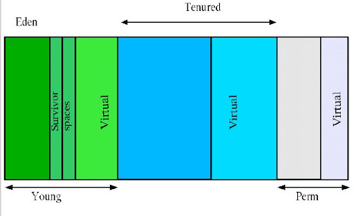
如上图所示，为Java堆中的各代分布

Young（年轻代）
年轻代分三个区一个Eden区，两个Survivor区大部分对象在Eden区中生成当Eden区满时，还存活的对象将被复制到Survivor区（两个中的一个），当这个Survivor区满时，此区的存活对象将被复制到另外一个Survivor区，当这个Survivor去也满了的时候，从第一个Survivor区复制过来的并且此时还存活的对象，将被复制年老区(Tenured)需要注意，Survivor的两个区是对称的，没先后关系，所以同一个区中可能同时存在从Eden复制过来 对象，和从前一个Survivor复制过来的对象，而复制到年老区的只有从第一个Survivor去过来的对象而且，Survivor区总有一个是空的Tenured（年老代）
年老代存放从年轻代存活的对象一般来说年老代存放的都是生命期较长的对象 Perm（持久代）
用于存放静态文件，如今Java类方法等持久代对垃圾回收没有显著影响，但是有些应用可能动态生成或者调用一些class，例如Hibernate等，在这种时候需要设置一个比较大的持久代空间来存放这些运行过程中新增的类持久代大小通过-XX:MaxPermSize=<N>进行设置
GC类型
GC有两种类型：Scavenge GC和Full GC Full GC
对整个堆进行整理，包括YoungTenured和PermFull GC比Scavenge GC要慢，因此应该尽可能减少Full GC有如下原因可能导致Full GC： Tenured被写满 Perm域被写满 System.gc()被显示调用 上一次GC之后Heap的各域分配策略动态变化

分代垃圾回收过程演示

目前的收集器主要有三种：串行收集器并行收集器并发收集器

串行收集器

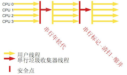
使用单线程处理所有垃圾回收工作，因为无需多线程交互，所以效率比较高但是，也无法使用多处理器的优势，所以此收集器适合单处理器机器当然，此收集器也可以用在小数据量（100M左右）情况下的多处理器机器上可以使用-XX:+UseSerialGC打开
并行收集器
对年轻代进行并行垃圾回收，因此可以减少垃圾回收时间一般在多线程多处理器机器上使用使用-XX:+UseParallelGC.打开并行收集器在J2SE5.0第六6更新上引入，在Java SE6.0中进行了增强--可以堆年老代进行并行收集如果年老代不使用并发收集的话，是使用单线程进行垃圾回收，因此会制约扩展能力使用-XX:+UseParallelOldGC打开 使用-XX:ParallelGCThreads=<N>设置并行垃圾回收的线程数此值可以设置与机器处理器数量相等 此收集器可以进行如下配置： 最大垃圾回收暂停:指定垃圾回收时的最长暂停时间，通过-XX:MaxGCPauseMillis=<N>指定<N>为毫秒.如果指定了此值的话，堆大小和垃圾回收相关参数会进行调整以达到指定值设定此值可能会减少应用的吞吐量 吞吐量:吞吐量为垃圾回收时间与非垃圾回收时间的比值，通过-XX:GCTimeRatio=<N>来设定，公式为1/（1+N）例如，-XX:GCTimeRatio=19时，表示5%的时间用于垃圾回收默认情况为99，即1%的时间用于垃圾回收并发收集器
可以保证大部分工作都并发进行（应用不停止），垃圾回收只暂停很少的时间，此收集器适合对响应时间要求比较高的中大规模应用使用-XX:+UseConcMarkSweepGC打开
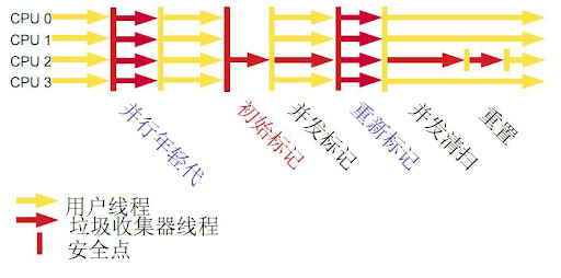 并发收集器主要减少年老代的暂停时间，他在应用不停止的情况下使用独立的垃圾回收线程，跟踪可达对象在每个年老代垃圾回收周期中，在收集初期并发收集器会对整个应用进行简短的暂停，在收集中还会再暂停一次第二次暂停会比第一次稍长，在此过程中多个线程同时进行垃圾回收工作 并发收集器使用处理器换来短暂的停顿时间在一个N个处理器的系统上，并发收集部分使用K/N个可用处理器进行回收，一般情况下1<=K<=N/4 在只有一个处理器的主机上使用并发收集器，设置为incremental mode模式也可获得较短的停顿时间 浮动垃圾：由于在应用运行的同时进行垃圾回收，所以有些垃圾可能在垃圾回收进行完成时产生，这样就造成了Floating Garbage，这些垃圾需要在下次垃圾回收周期时才能回收掉所以，并发收集器一般需要20%的预留空间用于这些浮动垃圾 Concurrent Mode Failure：并发收集器在应用运行时进行收集，所以需要保证堆在垃圾回收的这段时间有足够的空间供程序使用，否则，垃圾回收还未完成，堆空间先满了这种情况下将会发生并发模式失败，此时整个应用将会暂停，进行垃圾回收 启动并发收集器：因为并发收集在应用运行时进行收集，所以必须保证收集完成之前有足够的内存空间供程序使用，否则会出现Concurrent Mode Failure通过设置-XX:CMSInitiatingOccupancyFraction=<N>指定还有多少剩余堆时开始执行并发收集小结 并行处理器：
 --适用情况：对吞吐量有高要求，多CPU对应用响应时间无要求的中大型应用举例：后台处理科学计算
 --缺点：应用响应时间可能较长 并发处理器：
 --适用情况：对响应时间有高要求，多CPU对应用响应时间有较高要求的中大型应用举例：Web服务器/应用服务器电信交换集成开发环境
三常见配置举例 堆大小设置
JVM 中最大堆大小有三方面限制：相关操作系统的数据模型（32-bt还是64-bit）限制；系统的可用虚拟内存限制；系统的可用物理内存限制32位系统下，一般限制在1.5G~2G；64为操作系统对内存无限制我在Windows Server 2003 系统，3.5G物理内存，JDK5.0下测试，最大可设置为1478m
典型设置： java -Xmx3550m -Xms3550m -Xmn2g -Xss128k
-Xmx3550m：设置JVM最大可用内存为3550M
-Xms3550m：设置JVM促使内存为3550m此值可以设置与-Xmx相同，以避免每次垃圾回收完成后JVM重新分配内存
-Xmn2g：设置年轻代大小为2G整个堆大小=年轻代大小 + 年老代大小 + 持久代大小持久代一般固定大小为64m，所以增大年轻代后，将会减小年老代大小此值对系统性能影响较大，Sun官方推荐配置为整个堆的3/8
-Xss128k：设置每个线程的堆栈大小JDK5.0以后每个线程堆栈大小为1M，以前每个线程堆栈大小为256K更具应用的线程所需内存大小进行调整在相同物理内存下，减小这个值能生成更多的线程但是操作系统对一个进程内的线程数还是有限制的，不能无限生成，经验值在3000~5000左右
java -Xmx3550m -Xms3550m -Xss128k -XX:NewRatio=4 -XX:SurvivorRatio=4 -XX:MaxPermSize=16m -XX:MaxTenuringThreshold=0
-XX:NewRatio=4:设置年轻代（包括Eden和两个Survivor区）与年老代的比值（除去持久代）设置为4，则年轻代与年老代所占比值为1：4，年轻代占整个堆栈的1/5
-XX:SurvivorRatio=4：设置年轻代中Eden区与Survivor区的大小比值设置为4，则两个Survivor区与一个Eden区的比值为2:4，一个Survivor区占整个年轻代的1/6
-XX:MaxPermSize=16m:设置持久代大小为16m
-XX:MaxTenuringThreshold=0：设置垃圾最大年龄如果设置为0的话，则年轻代对象不经过Survivor区，直接进入年老代对于年老代比较多的应用，可以提高效率如果将此值设置为一个较大值，则年轻代对象会在Survivor区进行多次复制，这样可以增加对象再年轻代的存活时间，增加在年轻代即被回收的概论回收器选择
JVM给了三种选择：串行收集器并行收集器并发收集器，但是串行收集器只适用于小数据量的情况，所以这里的选择主要针对并行收集器和并发收集器默认情况下，JDK5.0以前都是使用串行收集器，如果想使用其他收集器需要在启动时加入相应参数JDK5.0以后，JVM会根据当前系统配置进行判断 吞吐量优先的并行收集器
如上文所述，并行收集器主要以到达一定的吞吐量为目标，适用于科学技术和后台处理等
典型配置： java -Xmx3800m -Xms3800m -Xmn2g -Xss128k -XX:+UseParallelGC -XX:ParallelGCThreads=20
-XX:+UseParallelGC：选择垃圾收集器为并行收集器此配置仅对年轻代有效即上述配置下，年轻代使用并发收集，而年老代仍旧使用串行收集
-XX:ParallelGCThreads=20：配置并行收集器的线程数，即：同时多少个线程一起进行垃圾回收此值最好配置与处理器数目相等
java -Xmx3550m -Xms3550m -Xmn2g -Xss128k -XX:+UseParallelGC -XX:ParallelGCThreads=20 -XX:+UseParallelOldGC
-XX:+UseParallelOldGC：配置年老代垃圾收集方式为并行收集JDK6.0支持对年老代并行收集
java -Xmx3550m -Xms3550m -Xmn2g -Xss128k -XX:+UseParallelGC  -XX:MaxGCPauseMillis=100
-XX:MaxGCPauseMillis=100:设置每次年轻代垃圾回收的最长时间，如果无法满足此时间，JVM会自动调整年轻代大小，以满足此值
java -Xmx3550m -Xms3550m -Xmn2g -Xss128k -XX:+UseParallelGC  -XX:MaxGCPauseMillis=100 -XX:+UseAdaptiveSizePolicy
-XX:+UseAdaptiveSizePolicy：设置此选项后，并行收集器会自动选择年轻代区大小和相应的Survivor区比例，以达到目标系统规定的最低相应时间或者收集频率等，此值建议使用并行收集器时，一直打开
响应时间优先的并发收集器
如上文所述，并发收集器主要是保证系统的响应时间，减少垃圾收集时的停顿时间适用于应用服务器电信领域等
典型配置： java -Xmx3550m -Xms3550m -Xmn2g -Xss128k -XX:ParallelGCThreads=20 -XX:+UseConcMarkSweepGC -XX:+UseParNewGC
-XX:+UseConcMarkSweepGC：设置年老代为并发收集测试中配置这个以后，-XX:NewRatio=4的配置失效了，原因不明所以，此时年轻代大小最好用-Xmn设置
-XX:+UseParNewGC:设置年轻代为并行收集可与CMS收集同时使用JDK5.0以上，JVM会根据系统配置自行设置，所以无需再设置此值 java -Xmx3550m -Xms3550m -Xmn2g -Xss128k -XX:+UseConcMarkSweepGC -XX:CMSFullGCsBeforeCompaction=5 -XX:+UseCMSCompactAtFullCollection
-XX:CMSFullGCsBeforeCompaction：由于并发收集器不对内存空间进行压缩整理，所以运行一段时间以后会产生碎片，使得运行效率降低此值设置运行多少次GC以后对内存空间进行压缩整理
-XX:+UseCMSCompactAtFullCollection：打开对年老代的压缩可能会影响性能，但是可以消除碎片
辅助信息
JVM提供了大量命令行参数，打印信息，供调试使用主要有以下一些： -XX:+PrintGC
输出形式：[GC 118250K->113543K(130112K), 0.0094143 secs]

                [Full GC 121376K->10414K(130112K), 0.0650971 secs]

-XX:+PrintGCDetails
输出形式：[GC [DefNew: 8614K->781K(9088K), 0.0123035 secs] 118250K->113543K(130112K), 0.0124633 secs]

                [GC [DefNew: 8614K->8614K(9088K), 0.0000665 secs][Tenured: 112761K->10414K(121024K), 0.0433488 secs] 121376K->10414K(130112K), 0.0436268 secs]

-XX:+PrintGCTimeStamps -XX:+PrintGC：PrintGCTimeStamps可与上面两个混合使用
输出形式：11.851: [GC 98328K->93620K(130112K), 0.0082960 secs]
-XX:+PrintGCApplicationConcurrentTime:打印每次垃圾回收前，程序未中断的执行时间可与上面混合使用
输出形式：Application time: 0.5291524 seconds
-XX:+PrintGCApplicationStoppedTime：打印垃圾回收期间程序暂停的时间可与上面混合使用
输出形式：Total time for which application threads were stopped: 0.0468229 seconds
-XX:PrintHeapAtGC:打印GC前后的详细堆栈信息
输出形式：
34.702: [GC {Heap before gc invocations=7:
 def new generation   total 55296K, used 52568K [0x1ebd0000, 0x227d0000, 0x227d0000)
eden space 49152K,  99% used [0x1ebd0000, 0x21bce430, 0x21bd0000)
from space 6144K,  55% used [0x221d0000, 0x22527e10, 0x227d0000)
  to   space 6144K,   0% used [0x21bd0000, 0x21bd0000, 0x221d0000)
 tenured generation   total 69632K, used 2696K [0x227d0000, 0x26bd0000, 0x26bd0000)
the space 69632K,   3% used [0x227d0000, 0x22a720f8, 0x22a72200, 0x26bd0000)
 compacting perm gen  total 8192K, used 2898K [0x26bd0000, 0x273d0000, 0x2abd0000)
   the space 8192K,  35% used [0x26bd0000, 0x26ea4ba8, 0x26ea4c00, 0x273d0000)
    ro space 8192K,  66% used [0x2abd0000, 0x2b12bcc0, 0x2b12be00, 0x2b3d0000)
    rw space 12288K,  46% used [0x2b3d0000, 0x2b972060, 0x2b972200, 0x2bfd0000)
34.735: [DefNew: 52568K->3433K(55296K), 0.0072126 secs] 55264K->6615K(124928K)Heap after gc invocations=8:
 def new generation   total 55296K, used 3433K [0x1ebd0000, 0x227d0000, 0x227d0000)
eden space 49152K,   0% used [0x1ebd0000, 0x1ebd0000, 0x21bd0000)
  from space 6144K,  55% used [0x21bd0000, 0x21f2a5e8, 0x221d0000)
  to   space 6144K,   0% used [0x221d0000, 0x221d0000, 0x227d0000)
 tenured generation   total 69632K, used 3182K [0x227d0000, 0x26bd0000, 0x26bd0000)
the space 69632K,   4% used [0x227d0000, 0x22aeb958, 0x22aeba00, 0x26bd0000)
 compacting perm gen  total 8192K, used 2898K [0x26bd0000, 0x273d0000, 0x2abd0000)
   the space 8192K,  35% used [0x26bd0000, 0x26ea4ba8, 0x26ea4c00, 0x273d0000)
    ro space 8192K,  66% used [0x2abd0000, 0x2b12bcc0, 0x2b12be00, 0x2b3d0000)
    rw space 12288K,  46% used [0x2b3d0000, 0x2b972060, 0x2b972200, 0x2bfd0000)
}
, 0.0757599 secs]
-Xloggc:filename:与上面几个配合使用，把相关日志信息记录到文件以便分析常见配置汇总 堆设置 -XX:NewSize=n:设置年轻代大小 -XX:NewRatio=n:设置年轻代和年老代的比值如:为3，表示年轻代与年老代比值为1：3，年轻代占整个年轻代年老代和的1/4 -XX:SurvivorRatio=n:年轻代中Eden区与两个Survivor区的比值注意Survivor区有两个如：3，表示Eden：Survivor=3：2，一个Survivor区占整个年轻代的1/5 -XX:MaxPermSize=n:设置持久代大小收集器设置 -XX:+UseSerialGC:设置串行收集器 -XX:+UseParallelGC:设置并行收集器 -XX:+UseParalledlOldGC:设置并行年老代收集器 -XX:+UseConcMarkSweepGC:设置并发收集器垃圾回收统计信息 -XX:+PrintGC -XX:+PrintGCDetails -XX:+PrintGCTimeStamps -Xloggc:filename并行收集器设置 -XX:ParallelGCThreads=n:设置并行收集器收集时使用的CPU数并行收集线程数 -XX:MaxGCPauseMillis=n:设置并行收集最大暂停时间 -XX:GCTimeRatio=n:设置垃圾回收时间占程序运行时间的百分比公式为1/(1+n)并发收集器设置 -XX:+CMSIncrementalMode:设置为增量模式适用于单CPU情况 -XX:ParallelGCThreads=n:设置并发收集器年轻代收集方式为并行收集时，使用的CPU数并行收集线程数
四调优总结 年轻代大小选择 响应时间优先的应用：尽可能设大，直到接近系统的最低响应时间限制（根据实际情况选择）在此种情况下，年轻代收集发生的频率也是最小的同时，减少到达年老代的对象 吞吐量优先的应用：尽可能的设置大，可能到达Gbit的程度因为对响应时间没有要求，垃圾收集可以并行进行，一般适合8CPU以上的应用年老代大小选择 响应时间优先的应用：年老代使用并发收集器，所以其大小需要小心设置，一般要考虑并发会话率和会话持续时间等一些参数如果堆设置小了，可以会造成内存碎片高回收频率以及应用暂停而使用传统的标记清除方式；如果堆大了，则需要较长的收集时间最优化的方案，一般需要参考以下数据获得： 减少年轻代和年老代花费的时间，一般会提高应用的效率
吞吐量优先的应用：一般吞吐量优先的应用都有一个很大的年轻代和一个较小的年老代原因是，这样可以尽可能回收掉大部分短期对象，减少中期的对象，而年老代尽存放长期存活对象较小堆引起的碎片问题
因为年老代的并发收集器使用标记清除算法，所以不会对堆进行压缩当收集器回收时，他会把相邻的空间进行合并，这样可以分配给较大的对象但是，当堆空间较小时，运行一段时间以后，就会出现碎片，如果并发收集器找不到足够的空间，那么并发收集器将会停止，然后使用传统的标记清除方式进行回收如果出现碎片，可能需要进行如下配置： -XX:+UseCMSCompactAtFullCollection：使用并发收集器时，开启对年老代的压缩 
五参考文献

http://java.sun.com/performance/reference/whitepapers/tuning.html#section4.1.3

http://www.oracle.com/technetwork/java/gc-tuning-5-138395.html

为什么要分代

分代的垃圾回收策略，是基于这样一个事实：不同的对象的生命周期是不一样的。因此，不同生命周期的对象可以采取不同的收集方式，以便提高回收效率。

在Java程序运行的过程中，会产生大量的对象，其中有些对象是与业务信息相关，比如Http请求中的Session对象、线程、Socket连接，这类对象跟业务直接挂钩，因此生命周期比较长。但是还有一些对象，主要是程序运行过程中生成的临时变量，这些对象生命周期会比较短，比如：String对象，由于其不变类的特性，系统会产生大量的这些对象，有些对象甚至只用一次即可回收。

试想，在不进行对象存活时间区分的情况下，每次垃圾回收都是对整个堆空间进行回收，花费时间相对会长，同时，因为每次回收都需要遍历所有存活对象，但实际上，对于生命周期长的对象而言，这种遍历是没有效果的，因为可能进行了很多次遍历，但是他们依旧存在。因此，分代垃圾回收采用分治的思想，进行代的划分，把不同生命周期的对象放在不同代上，不同代上采用最适合它的垃圾回收方式进行回收。

如何分代

如图所示：

 

虚拟机中的共划分为三个代：年轻代（Young Generation）、年老点（Old Generation）和持久代（Permanent Generation）。其中持久代主要存放的是Java类的类信息，与垃圾收集要收集的Java对象关系不大。年轻代和年老代的划分是对垃圾收集影响比较大的。

年轻代:

所有新生成的对象首先都是放在年轻代的。年轻代的目标就是尽可能快速的收集掉那些生命周期短的对象。年轻代分三个区。一个Eden区，两个Survivor区(一般而言)。大部分对象在Eden区中生成。当Eden区满时，还存活的对象将被复制到Survivor区（两个中的一个），当这个Survivor区满时，此区的存活对象将被复制到另外一个Survivor区，当这个Survivor去也满了的时候，从第一个Survivor区复制过来的并且此时还存活的对象，将被复制“年老区(Tenured)”。需要注意，Survivor的两个区是对称的，没先后关系，所以同一个区中可能同时存在从Eden复制过来 对象，和从前一个Survivor复制过来的对象，而复制到年老区的只有从第一个Survivor去过来的对象。而且，Survivor区总有一个是空的。同时，根据程序需要，Survivor区是可以配置为多个的（多于两个），这样可以增加对象在年轻代中的存在时间，减少被放到年老代的可能。

年老代:

在年轻代中经历了N次垃圾回收后仍然存活的对象，就会被放到年老代中。因此，可以认为年老代中存放的都是一些生命周期较长的对象。

持久代:

用于存放静态文件，如今Java类、方法等。持久代对垃圾回收没有显著影响，但是有些应用可能动态生成或者调用一些class，例如Hibernate等，在这种时候需要设置一个比较大的持久代空间来存放这些运行过程中新增的类。持久代大小通过-XX:MaxPermSize=<N>进行设置。

什么情况下触发垃圾回收

由于对象进行了分代处理，因此垃圾回收区域、时间也不一样。GC有两种类型：Scavenge GC和Full GC。

Scavenge GC

一般情况下，当新对象生成，并且在Eden申请空间失败时，就会触发Scavenge GC，对Eden区域进行GC，清除非存活对象，并且把尚且存活的对象移动到Survivor区。然后整理Survivor的两个区。这种方式的GC是对年轻代的Eden区进行，不会影响到年老代。因为大部分对象都是从Eden区开始的，同时Eden区不会分配的很大，所以Eden区的GC会频繁进行。因而，一般在这里需要使用速度快、效率高的算法，使Eden去能尽快空闲出来。

Full GC

• JVM基础概念总结：数据类型、堆与栈
• JVM概念之Java对象的大小与引用类型
• 漫谈Java理念的转变与JVM的五大优势
• 漫谈JVM的基本垃圾回收算法
• JVM垃圾回收面临的问题

对整个堆进行整理，包括Young、Tenured和Perm。Full GC因为需要对整个对进行回收，所以比Scavenge GC要慢，因此应该尽可能减少Full GC的次数。在对JVM调优的过程中，很大一部分工作就是对于FullGC的调节。有如下原因可能导致Full GC：

· 年老代（Tenured）被写满

· 持久代（Perm）被写满

· System.gc()被显示调用

·上一次GC之后Heap的各域分配策略动态变化