模式识别经常用到的距离测度

来源：互联网发布：c#书籍推荐知乎编辑：程序博客网时间：2024/05/01 07:09

http://repository.cmu.edu/cgi/viewcontent.cgi?article=1447&context=robotics

1. Euclidean distance

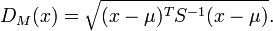
2. Mahalanobis distance

Please refer to the following explenation as well as the attached file which is even clearer

Distance is not always what it seems

You can generalize these ideas to the multivariate normal distribution.The following graph shows simulated bivariate normal data that is overlaid withprediction ellipses. The ellipses in the graph are the 10% (innermost), 20%, ..., and 90% (outermost) prediction ellipses for the bivariate normal distribution that generated the data. The prediction ellipses are contours of the bivariate normal density function. The probability density is high for ellipses near the origin, such as the 10% prediction ellipse. The density is low for ellipses are further away, such as the 90% prediction ellipse.

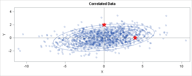
In the graph, two observations are displayed by using red stars as markers. The first observation is at the coordinates (4,0), whereas the second is at (0,2). The question is: which marker is closer to the origin? (The origin is the multivariate center of this distribution.)

The answer is, "It depends how you measure distance." The Euclidean distances are 4 and 2, respectively, so you might conclude that the point at (0,2) is closer to the origin. However, for this distribution, the variance in the Y direction is less than the variance in the X direction, so in some sense the point (0,2) is "more standard deviations" away from the origin than (4,0) is.</p

Notice the position of the two observations relative to the ellipses. The point (0,2) is located at the 90% prediction ellipse, whereas the point at (4,0) is located at about the 75% prediction ellipse. What does this mean? It means that the point at (4,0) is "closer" to the origin in the sense that you are more likely to observe an observation near (4,0) than to observe one near (0,2). The probability density is higher near (4,0) than it is near (0,2).

In this sense, prediction ellipses are a multivariate generalization of "units of standard deviation." You can use the bivariate probability contours to compare distances to the bivariate mean. A pointp is closer than a pointq if the contour that contains p is nested within the contour that containsq.

Defining the Mahalanobis distance

You can use the probability contours to define the Mahalanobis distance.The Mahalanobis distance has the following properties:

It accounts for the fact that the variances in each direction are different.
It accounts for the covariance between variables.
It reduces to the familiar Euclidean distance for uncorrelated variables with unit variance.

For univariate normal data, the univariate z-score standardizes the distribution (so that it has mean 0 and unit variance) and gives a dimensionless quantity that specifies the distance from an observation to the mean in terms of the scale of the data. For multivariate normal data with mean μ and covariance matrix Σ, you can decorrelate the variables and standardize the distribution by applying the Cholesky transformationz = L^-1(x - μ), whereL is the Cholesky factor of Σ, Σ=LL^T.

After transforming the data, you can compute the standard Euclidian distance from the pointz to the origin. In order to get rid of square roots, I'll compute the square of the Euclidean distance, which is dist²(z,0) = z^Tz.This measures how far from the origin a point is, and it is the multivariate generalization of a z-score.

You can rewrite z^Tz in terms of the original correlated variables. The squared distance Mahal²(x,μ) is
= z^T z
= (L^-1(x - μ))^T (L^-1(x - μ))
= (x - μ)^T (LL^T)^-1 (x - μ)
= (x - μ)^T Σ ^-1 (x - μ)
The last formula is the definition of the squared Mahalanobis distance. The derivation uses several matrix identities such as (AB)^T = B^TA^T, (AB)^-1 = B^-1A^-1, and (A^-1)^T = (A^T)^-1. Notice that if Σ is the identity matrix, then the Mahalanobis distance reduces to the standard Euclidean distance betweenx and μ.

The Mahalanobis distance accounts for the variance of each variable and the covariance between variables. Geometrically, it does this by transforming the data into standardized uncorrelated data and computing the ordinary Euclidean distance for the transformed data. In this way, the Mahalanobis distance is like a univariate z-score: it provides a way to measure distances that takes into account the scale of the data.

--------

Formally, the Mahalanobis distance of a multivariate vector $x = ( x_1, x_2, x_3, \dots, x_N )^T$ from a group of values with mean $\mu = ( \mu_1, \mu_2, \mu_3, \dots , \mu_N )^T$ andcovariance matrix $S$ is defined as:

$D_M(x) = \sqrt{(x - \mu)^T S^{-1} (x-\mu)}.\,$ ^[2]

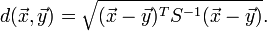
Mahalanobis distance (or "generalized squared interpoint distance" for its squared value^[3]) can also be defined as a dissimilarity measure between two random vectors $\vec{x}$ and $\vec{y}$ of the samedistribution with thecovariance matrix $S$ :

$d(\vec{x},\vec{y})=\sqrt{(\vec{x}-\vec{y})^T S^{-1} (\vec{x}-\vec{y})}.\,$

If the covariance matrix is the identity matrix, the Mahalanobis distance reduces to theEuclidean distance. If the covariance matrix isdiagonal, then the resulting distance measure is called thenormalized Euclidean distance:

$d(\vec{x},\vec{y})=\sqrt{\sum_{i=1}^N {(x_i - y_i)^2 \over s_{i}^2}},$

where $s_{i}$ is thestandard deviation of the $x_i$ and $y_i$ over the sample set.

Intuitive explanation

Consider the problem of estimating the probability that a test point in N-dimensionalEuclidean space belongs to a set, where we are given sample points that definitely belong to that set. Our first step would be to find the average or center of mass of the sample points. Intuitively, the closer the point in question is to this center of mass, the more likely it is to belong to the set.

However, we also need to know if the set is spread out over a large range or a small range, so that we can decide whether a given distance from the center is noteworthy or not. The simplistic approach is to estimate thestandard deviation of the distances of the sample points from the center of mass. If the distance between the test point and the center of mass is less than one standard deviation, then we might conclude that it is highly probable that the test point belongs to the set. The further away it is, the more likely that the test point should not be classified as belonging to the set.

This intuitive approach can be made quantitative by defining the normalized distance between the test point and the set to be ${x - \mu} \over \sigma$ . By plugging this into the normal distribution we can derive the probability of the test point belonging to the set.

The drawback of the above approach was that we assumed that the sample points are distributed about the center of mass in a spherical manner. Were the distribution to be decidedly non-spherical, for instance ellipsoidal, then we would expect the probability of the test point belonging to the set to depend not only on the distance from the center of mass, but also on the direction. In those directions where the ellipsoid has a short axis the test point must be closer, while in those where the axis is long the test point can be further away from the center.

Putting this on a mathematical basis, the ellipsoid that best represents the set's probability distribution can be estimated by building the covariance matrix of the samples. The Mahalanobis distance is simply the distance of the test point from the center of mass divided by the width of the ellipsoid in the direction of the test point.

3. Hamming distance

4. Hausdorff distance

Definition

Components of the calculation of the Hausdorff distance between the green line X and the blue line Y.

Let X and Y be two non-empty subsets of a metric space (M, d). We define their Hausdorff distanced_H(X, Y) by

$d_{\mathrm H}(X,Y) = \max\{\,\sup_{x \in X} \inf_{y \in Y} d(x,y),\, \sup_{y \in Y} \inf_{x \in X} d(x,y)\,\}\mbox{,} \!$

where sup represents the supremum and inf the infimum.

Equivalently

$d_H(X,Y) = \inf\{\epsilon > 0\,;\ X \subseteq Y_\epsilon \ \mbox{and}\ Y \subseteq X_\epsilon\}$ ,^[2]

where

$X_\epsilon := \bigcup_{x \in X} \{z \in M\,;\ d(z,x) \leq \epsilon\}$ ,

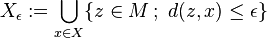
that is, the set of all points within $\epsilon$ of the set $X$ (sometimes called the $\epsilon$ -fattening of $X$ or a generalized ball of radius $\epsilon$ around $X$ ).

[edit]Remark

It is not true in general that if $d_H(X,Y) = \epsilon$ , then

$X\subseteq Y_\epsilon \ \mbox{and} \ Y\subseteq X_\epsilon$ .

For instance, consider the metric space of the real numbers $\mathbb{R}$ with the usual metric $d$ induced by the absolute value,

$d(x,y) := |y - x|, \quad x,y \in \mathbb{R}$ .

Take

$X := \{1/n\,;\ n \in \mathbb{N}\} \quad \mbox{and} \quad Y := \{-1/n\,;\ n \in \mathbb{N}\}$ .

Then $d_H(X,Y) = 1\$ . However $X \nsubseteq Y_1$ because $Y_1 \subset [-2,1)\$ , but $1 \in X$ .

[edit]Properties

In general, d_H(X,Y) may be infinite. If bothX and Y are bounded, then d_H(X,Y) is guaranteed to be finite.

We have d_H(X,Y) = 0 if and only if X andY have the same closure.

On the set of all non-empty subsets of M, d_H yields an extendedpseudometric.

On the set F(M) of all non-empty compact subsets of M,d_H is a metric. If M is complete, then so is F(M).^[3] IfM is compact, then so is F(M). The topology of F(M) depends only on the topology of M, not on the metricd.

5. PCA Distance measures based on PCA or
eigenspaces are perhaps the most popular. The underlying
assumption when using PCA is that the measurement
data can be explained (modulo noise) by a small dimensional linear subspace of

6. Discriminative analysis, of which LDA [3, 16]
is the most popular, on the other hand explicitly tries to
find discriminative distance measures that separate the different
classes from each other as much as possible

7. Support Vector Machines that
maximize the margin between different classes

8. Bayesian
approaches to classification estimates probability density
models for each class and classifies an input query using the
Bayes rule. For the two class case, the log-odds ratio can be
considered to be a discriminative distance measure

such approaches typically suffer
from the need to specify an appropriate model for each
class as well as estimating such models reliably from data