Histograms of Oriented Gradients (HOG)理解和源码
来源:互联网 发布:3d免费犀牛怎么编程 编辑:程序博客网 时间:2024/05/22 16:27
HOG descriptors 是应用在计算机视觉和图像处理领域,用于目标检测的特征描述器。这项技术是用来计算局部图像梯度的方向信息的统计值。这种方法跟边缘方向直方图(edge orientation histograms)、尺度不变特征变换(scale-invariant feature transform descriptors) 以及形状上下文方法( shape contexts)有很多相似之处,但与它们的不同点是:HOG描述器是在一个网格密集的大小统一的细胞单元(dense grid of uniformly spaced cells)上计算,而且为了提高性能,还采用了重叠的局部对比度归一化(overlapping local contrast normalization)技术。
这篇文章的作者Navneet Dalal和Bill Triggs是法国国家计算机技术和控制研究所French National Institute for Research in Computer Science and Control (INRIA)的研究员。他们在这篇文章中首次提出了HOG方法。这篇文章被发表在2005年的CVPR上。他们主要是将这种方法应用在静态图像中的行人 检测上,但在后来,他们也将其应用在电影和视频中的行人检测,以及静态图像中的车辆和常见动物的检测。
HOG描述器最重要的思想是:在一副 图像中,局部目标的表象和形状(appearance and shape)能够被梯度或边缘的方向密度分布很好地描述。具体的实现方法是:首先将图像分成小的连通区域,我们把它叫细胞单元。然后采集细胞单元中各像素 点的梯度的或边缘的方向直方图。最后把这些直方图组合起来就可以构成特征描述器。为了提高性能,我们还可以把这些局部直方图在图像的更大的范围内(我们把 它叫区间或block)进行对比度归一化(contrast-normalized),所采用的方法是:先计算各直方图在这个区间(block)中的密 度,然后根据这个密度对区间中的各个细胞单元做归一化。通过这个归一化后,能对光照变化和阴影获得更好的效果。
与其他的特征描述方法相 比,HOG描述器后很多优点。首先,由于HOG方法是在图像的局部细胞单元上操作,所以它对图像几何的(geometric)和光学的 (photometric)形变都能保持很好的不变性,这两种形变只会出现在更大的空间领域上。其次,作者通过实验发现,在粗的空域抽样(coarse spatial sampling)、精细的方向抽样(fine orientation sampling)以及较强的局部光学归一化(strong local photometric normalization)等条件下,只要行人大体上能够保持直立的姿势,就容许行人有一些细微的肢体动作,这些细微的动作可以被忽略而不影响检测效 果。综上所述,HOG方法是特别适合于做图像中的行人检测的。
上图是作者做的行人检测试验,其中(a)表示所有训练图像集 的平均梯度(average gradient across their training images);(b)和(c)分别表示:图像中每一个区间(block)上的最大最大正、负SVM权值;(d)表示一副测试图像;(e)计算完R- HOG后的测试图像;(f)和(g)分别表示被正、负SVM权值加权后的R-HOG图像。
算法的实现:
色彩和伽马归一化 (color and gamma normalization)
作者分别在灰度空间、RGB色彩空间和LAB色彩空间上对图像进行色彩和 伽马归一化,但实验结果显示,这个归一化的预处理工作对最后的结果没有影响,原因可能是:在后续步骤中也有归一化的过程,那些过程可以取代这个预处理的归 一化。所以,在实际应用中,这一步可以省略。
梯度的计算(Gradient computation)
最常用的方法是:简单 地使用一个一维的离散微分模板(1-D centered point discrete derivative mask)在一个方向上或者同时在水平和垂直两个方向上对图像进行处理,更确切地说,这个方法需要使用下面的滤波器核滤除图像中的色彩或变化剧烈的数据 (color or intensity data)
作者也尝试了其他一些更复杂的模板,如3×3 Sobel 模板,或对角线模板(diagonal masks),但是在这个行人检测的实验中,这些复杂模板的表现都较差,所以作者的结论是:模板越简单,效果反而越好。作者也尝试了在使用微分模板前加入 一个高斯平滑滤波,但是这个高斯平滑滤波的加入使得检测效果更差,原因是:许多有用的图像信息是来自变化剧烈的边缘,而在计算梯度之前加入高斯滤波会把这 些边缘滤除掉。
构建方向的直方图(creating the orientation histograms)
第三步就是为 图像的每个细胞单元构建梯度方向直方图。细胞单元中的每一个像素点都为某个基于方向的直方图通道(orientation-based histogram channel)投票。投票是采取加权投票(weighted voting)的方式,即每一票都是带权值的,这个权值是根据该像素点的梯度幅度计算出来。可以采用幅值本身或者它的函数来表示这个权值,实际测试表明: 使用幅值来表示权值能获得最佳的效果,当然,也可以选择幅值的函数来表示,比如幅值的平方根(square root)、幅值的平方(square of the gradient magnitude)、幅值的截断形式(clipped version of the magnitude)等。细胞单元可以是矩形的(rectangular),也可以是星形的(radial)。直方图通道是平均分布在0-1800(无 向)或0-3600(有向)范围内。作者发现,采用无向的梯度和9个直方图通道,能在行人检测试验中取得最佳的效果。
把细胞单元组 合成大的区间(grouping the cells together into larger blocks)
由于局部光照的变化 (variations of illumination)以及前景-背景对比度(foreground-background contrast)的变化,使得梯度强度(gradient strengths)的变化范围非常大。这就需要对梯度强度做归一化,作者采取的办法是:把各个细胞单元组合成大的、空间上连通的区间(blocks)。 这样以来,HOG描述器就变成了由各区间所有细胞单元的直方图成分所组成的一个向量。这些区间是互有重叠的,这就意味着:每一个细胞单元的输出都多次作用 于最终的描述器。区间有两个主要的几何形状——矩形区间(R-HOG)和环形区间(C-HOG)。R-HOG区间大体上是一些方形的格子,它可以有三个参 数来表征:每个区间中细胞单元的数目、每个细胞单元中像素点的数目、每个细胞的直方图通道数目。作者通过实验表明,行人检测的最佳参数设置是:3×3细胞 /区间、6×6像素/细胞、9个直方图通道。作者还发现,在对直方图做处理之前,给每个区间(block)加一个高斯空域窗口(Gaussian spatial window)是非常必要的,因为这样可以降低边缘的周围像素点(pixels around the edge)的权重。
R- HOG跟SIFT描述器看起来很相似,但他们的不同之处是:R-HOG是在单一尺度下、密集的网格内、没有对方向排序的情况下被计算出来(are computed in dense grids at some single scale without orientation alignment);而SIFT描述器是在多尺度下、稀疏的图像关键点上、对方向排序的情况下被计算出来(are computed at sparse scale-invariant key image points and are rotated to align orientation)。补充一点,R-HOG是各区间被组合起来用于对空域信息进行编码(are used in conjunction to encode spatial form information),而SIFT的各描述器是单独使用的(are used singly)。
C- HOG区间(blocks)有两种不同的形式,它们的区别在于:一个的中心细胞是完整的,一个的中心细胞是被分割的。如右图所示:
作者发现 C-HOG的这两种形式都能取得相同的效果。C-HOG区间(blocks)可以用四个参数来表征:角度盒子的个数(number of angular bins)、半径盒子个数(number of radial bins)、中心盒子的半径(radius of the center bin)、半径的伸展因子(expansion factor for the radius)。通过实验,对于行人检测,最佳的参数设置为:4个角度盒子、2个半径盒子、中心盒子半径为4个像素、伸展因子为2。前面提到过,对于R- HOG,中间加一个高斯空域窗口是非常有必要的,但对于C-HOG,这显得没有必要。C-HOG看起来很像基于形状上下文(Shape Contexts)的方法,但不同之处是:C-HOG的区间中包含的细胞单元有多个方向通道(orientation channels),而基于形状上下文的方法仅仅只用到了一个单一的边缘存在数(edge presence count)。
区间归一化 (Block normalization)
作者采用了四中不同的方法对区间进行归一化,并对结果进行了比较。引入v表示一个还没有被归一 化的向量,它包含了给定区间(block)的所有直方图信息。| | vk | |表示v的k阶范数,这里的k去1、2。用e表示一个很小的常数。这时,归一化因子可以表示如下:
L2-norm:
L1-norm:
L1-sqrt:
还 有第四种归一化方式:L2-Hys,它可以通过先进行L2-norm,对结果进行截短(clipping),然后再重新归一化得到。作者发现:采用L2- Hys L2-norm 和 L1-sqrt方式所取得的效果是一样的,L1-norm稍微表现出一点点不可靠性。但是对于没有被归一化的数据来说,这四种方法都表现出来显着的改进。
SVM 分类器(SVM classifier)
最后一步就是把提取的HOG特征输入到SVM分类器中,寻找一个最优超平面作为决策函数。作者采用 的方法是:使用免费的SVMLight软件包加上HOG分类器来寻找测试图像中的行人。
Matlab源码:见TimeHandle的blog
转自:http://www.zhizhihu.com/html/y2010/1690.html
Histograms of Oriented Gradients (HOG)特征 MATLAB 计算
- function F = hogcalculator(img, cellpw, cellph, nblockw, nblockh,...
- nthet, overlap, isglobalinterpolate, issigned, normmethod)
- % HOGCALCULATOR calculate R-HOG feature vector of an input image using the
- % procedure presented in Dalal and Triggs's paper in CVPR 2005.
- %
- % Author: timeHandle
- % Time: March 24, 2010
- % May 12,2010 update.
- %
- % this copy of code is written for my personal interest, which is an
- % original and inornate realization of [Dalal CVPR2005]'s algorithm
- % without any optimization. I just want to check whether I understand
- % the algorithm really or not, and also do some practices for knowing
- % matlab programming more well because I could be called as 'novice'.
- % OpenCV 2.0 has realized Dalal's HOG algorithm which runs faster
- % than mine without any doubt, ╮(╯▽╰)╭ . Ronan pointed a error in
- % the code,thanks for his correction. Note that at the end of this
- % code, there are some demonstration code,please remove in your work.
- %
- % F = hogcalculator(img, cellpw, cellph, nblockw, nblockh,
- % nthet, overlap, isglobalinterpolate, issigned, normmethod)
- %
- % IMG:
- % IMG is the input image.
- %
- % CELLPW, CELLPH:
- % CELLPW and CELLPH are cell's pixel width and height respectively.
- %
- % NBLOCKW, NBLCOKH:
- % NBLOCKW and NBLCOKH are block size counted by cells number in x and
- % y directions respectively.
- %
- % NTHET, ISSIGNED:
- % NTHET is the number of the bins of the histogram of oriented
- % gradient. The histogram of oriented gradient ranges from 0 to pi in
- % 'unsigned' condition while to 2*pi in 'signed' condition, which can
- % be specified through setting the value of the variable ISSIGNED by
- % the string 'unsigned' or 'signed'.
- %
- % OVERLAP:
- % OVERLAP is the overlap proportion of two neighboring block.
- %
- % ISGLOBALINTERPOLATE:
- % ISGLOBALINTERPOLATE specifies whether the trilinear interpolation
- % is done in a single global 3d histogram of the whole detecting
- % window by the string 'globalinterpolate' or in each local 3d
- % histogram corresponding to respective blocks by the string
- % 'localinterpolate' which is in strict accordance with the procedure
- % proposed in Dalal's paper. Interpolating in the whole detecting
- % window requires the block's sliding step to be an integral multiple
- % of cell's width and height because the histogram is fixing before
- % interpolate. In fact here the so called 'global interpolation' is
- % a notation given by myself. at first the spatial interpolation is
- % done without any relevant to block's slide position, but when I was
- % doing calculation while OVERLAP is 0.75, something occurred and
- % confused me o__O"… . This let me find that the operation I firstly
- % did is different from which mentioned in Dalal's paper. But this
- % does not mean it is incorrect ^◎^, so I reserve this. As for name,
- % besides 'global interpolate', any others would be all ok, like 'Lady GaGa'
- % or what else, :-).
- %
- % NORMMETHOD:
- % NORMMETHOD is the block histogram normalized method which can be
- % set as one of the following strings:
- % 'none', which means non-normalization;
- % 'l1', which means L1-norm normalization;
- % 'l2', which means L2-norm normalization;
- % 'l1sqrt', which means L1-sqrt-norm normalization;
- % 'l2hys', which means L2-hys-norm normalization.
- % F:
- % F is a row vector storing the final histogram of all of the blocks
- % one by one in a top-left to bottom-right image scan manner, the
- % cells histogram are stored in the same manner in each block's
- % section of F.
- %
- % Note that CELLPW*NBLOCKW and CELLPH*NBLOCKH should be equal to IMG's
- % width and height respectively.
- %
- % Here is a demonstration, which all of parameters are set as the
- % best value mentioned in Dalal's paper when the window detected is 128*64
- % size(128 rows, 64 columns):
- % F = hogcalculator(window, 8, 8, 2, 2, 9, 0.5,
- % 'localinterpolate', 'unsigned', 'l2hys');
- % Also the function can be called like:
- % F = hogcalculator(window);
- % the other parameters are all set by using the above-mentioned "dalal's
- % best value" as default.
- %
- if nargin < 2
- % set default parameters value.
- cellpw = 8;
- cellph = 8;
- nblockw = 2;
- nblockh = 2;
- nthet = 9;
- overlap = 0.5;
- isglobalinterpolate = 'localinterpolate';
- issigned = 'unsigned';
- normmethod = 'l2hys';
- else
- if nargin < 10
- error('Input parameters are not enough.');
- end
- end
- % check parameters's validity.
- [M, N, K] = size(img);
- if mod(M,cellph*nblockh) ~= 0
- error('IMG''s height should be an integral multiple of CELLPH*NBLOCKH.');
- end
- if mod(N,cellpw*nblockw) ~= 0
- error('IMG''s width should be an integral multiple of CELLPW*NBLOCKW.');
- end
- if mod((1-overlap)*cellpw*nblockw, cellpw) ~= 0 ||...
- mod((1-overlap)*cellph*nblockh, cellph) ~= 0
- str1 = 'Incorrect OVERLAP or ISGLOBALINTERPOLATE parameter';
- str2 = ', slide step should be an intergral multiple of cell size';
- error([str1, str2]);
- end
- % set the standard deviation of gaussian spatial weight window.
- delta = cellpw*nblockw * 0.5;
- % calculate gradient scale matrix.
- hx = [-1,0,1];
- hy = -hx';
- gradscalx = imfilter(double(img),hx);
- gradscaly = imfilter(double(img),hy);
- %
- if K > 1
- % gradscalx = max(max(gradscalx(:,:,1),gradscalx(:,:,2)), gradscalx(:,:,3));
- % gradscaly = max(max(gradscaly(:,:,1),gradscaly(:,:,2)), gradscaly(:,:,3));
- maxgrad = sqrt(double(gradscalx.*gradscalx + gradscaly.*gradscaly));
- [gradscal, gidx] = max(maxgrad,[],3);
- gxtemp = zeros(M,N);
- gytemp = gxtemp;
- for kn = 1:K
- [rowidx, colidx] = ind2sub(size(gidx),find(gidx==kn));
- gxtemp(rowidx, colidx) = gradscalx(rowidx,colidx,kn);
- gytemp(rowidx, colidx) =gradscaly(rowidx,colidx,kn);
- end
- gradscalx = gxtemp;
- gradscaly = gytemp;
- else
- gradscal = sqrt(double(gradscalx.*gradscalx + gradscaly.*gradscaly));
- end
- % calculate gradient orientation matrix.
- % plus small number for avoiding dividing zero.
- gradscalxplus = gradscalx+ones(size(gradscalx))*0.0001;
- gradorient = zeros(M,N);
- % unsigned situation: orientation region is 0 to pi.
- if strcmp(issigned, 'unsigned') == 1
- gradorient =...
- atan(gradscaly./gradscalxplus) + pi/2;
- or = 1;
- else
- % signed situation: orientation region is 0 to 2*pi.
- if strcmp(issigned, 'signed') == 1
- idx = find(gradscalx >= 0 & gradscaly >= 0);
- gradorient(idx) = atan(gradscaly(idx)./gradscalxplus(idx));
- idx = find(gradscalx < 0);
- gradorient(idx) = atan(gradscaly(idx)./gradscalxplus(idx)) + pi;
- idx = find(gradscalx >= 0 & gradscaly < 0);
- gradorient(idx) = atan(gradscaly(idx)./gradscalxplus(idx)) + 2*pi;
- or = 2;
- else
- error('Incorrect ISSIGNED parameter.');
- end
- end
- % calculate block slide step.
- xbstride = cellpw*nblockw*(1-overlap);
- ybstride = cellph*nblockh*(1-overlap);
- xbstridend = N - cellpw*nblockw + 1;
- ybstridend = M - cellph*nblockh + 1;
- % calculate the total blocks number in the window detected, which is
- % ntotalbh*ntotalbw.
- ntotalbh = ((M-cellph*nblockh)/ybstride)+1;
- ntotalbw = ((N-cellpw*nblockw)/xbstride)+1;
- % generate the matrix hist3dbig for storing the 3-dimensions histogram. the
- % matrix covers the whole image in the 'globalinterpolate' condition or
- % covers the local block in the 'localinterpolate' condition. The matrix is
- % bigger than the area where it covers by adding additional elements
- % (corresponding to the cells) to the surround for calculation convenience.
- if strcmp(isglobalinterpolate, 'globalinterpolate') == 1
- ncellx = N / cellpw;
- ncelly = M / cellph;
- hist3dbig = zeros(ncelly+2, ncellx+2, nthet+2);
- F = zeros(1, (M/cellph-1)*(N/cellpw-1)*nblockw*nblockh*nthet);
- glbalinter = 1;
- else
- if strcmp(isglobalinterpolate, 'localinterpolate') == 1
- hist3dbig = zeros(nblockh+2, nblockw+2, nthet+2);
- F = zeros(1, ntotalbh*ntotalbw*nblockw*nblockh*nthet);
- glbalinter = 0;
- else
- error('Incorrect ISGLOBALINTERPOLATE parameter.')
- end
- end
- % generate the matrix for storing histogram of one block;
- sF = zeros(1, nblockw*nblockh*nthet);
- % generate gaussian spatial weight.
- [gaussx, gaussy] = meshgrid(0:(cellpw*nblockw-1), 0:(cellph*nblockh-1));
- weight = exp(-((gaussx-(cellpw*nblockw-1)/2)...
- .*(gaussx-(cellpw*nblockw-1)/2)+(gaussy-(cellph*nblockh-1)/2)...
- .*(gaussy-(cellph*nblockh-1)/2))/(delta*delta));
- % vote for histogram. there are two situations according to the interpolate
- % condition('global' interpolate or local interpolate). The hist3d which is
- % generated from the 'bigger' matrix hist3dbig is the final histogram.
- if glbalinter == 1
- xbstep = nblockw*cellpw;
- ybstep = nblockh*cellph;
- else
- xbstep = xbstride;
- ybstep = ybstride;
- end
- % block slide loop
- for btly = 1:ybstep:ybstridend
- for btlx = 1:xbstep:xbstridend
- for bi = 1:(cellph*nblockh)
- for bj = 1:(cellpw*nblockw)
- i = btly + bi - 1;
- j = btlx + bj - 1;
- gaussweight = weight(bi,bj);
- gs = gradscal(i,j);
- go = gradorient(i,j);
- if glbalinter == 1
- jorbj = j;
- iorbi = i;
- else
- jorbj = bj;
- iorbi = bi;
- end
- % calculate bin index of hist3dbig
- binx1 = floor((jorbj-1+cellpw/2)/cellpw) + 1;
- biny1 = floor((iorbi-1+cellph/2)/cellph) + 1;
- binz1 = floor((go+(or*pi/nthet)/2)/(or*pi/nthet)) + 1;
- if gs < 1E-5
- continue;
- end
- binx2 = binx1 + 1;
- biny2 = biny1 + 1;
- binz2 = binz1 + 1;
- x1 = (binx1-1.5)*cellpw + 0.5;
- y1 = (biny1-1.5)*cellph + 0.5;
- z1 = (binz1-1.5)*(or*pi/nthet);
- % trilinear interpolation.
- hist3dbig(biny1,binx1,binz1) =...
- hist3dbig(biny1,binx1,binz1) + gs*gaussweight...
- * (1-(jorbj-x1)/cellpw)*(1-(iorbi-y1)/cellph)...
- *(1-(go-z1)/(or*pi/nthet));
- hist3dbig(biny1,binx1,binz2) =...
- hist3dbig(biny1,binx1,binz2) + gs*gaussweight...
- * (1-(jorbj-x1)/cellpw)*(1-(iorbi-y1)/cellph)...
- *((go-z1)/(or*pi/nthet));
- hist3dbig(biny2,binx1,binz1) =...
- hist3dbig(biny2,binx1,binz1) + gs*gaussweight...
- * (1-(jorbj-x1)/cellpw)*((iorbi-y1)/cellph)...
- *(1-(go-z1)/(or*pi/nthet));
- hist3dbig(biny2,binx1,binz2) =...
- hist3dbig(biny2,binx1,binz2) + gs*gaussweight...
- * (1-(jorbj-x1)/cellpw)*((iorbi-y1)/cellph)...
- *((go-z1)/(or*pi/nthet));
- hist3dbig(biny1,binx2,binz1) =...
- hist3dbig(biny1,binx2,binz1) + gs*gaussweight...
- * ((jorbj-x1)/cellpw)*(1-(iorbi-y1)/cellph)...
- *(1-(go-z1)/(or*pi/nthet));
- hist3dbig(biny1,binx2,binz2) =...
- hist3dbig(biny1,binx2,binz2) + gs*gaussweight...
- * ((jorbj-x1)/cellpw)*(1-(iorbi-y1)/cellph)...
- *((go-z1)/(or*pi/nthet));
- hist3dbig(biny2,binx2,binz1) =...
- hist3dbig(biny2,binx2,binz1) + gs*gaussweight...
- * ((jorbj-x1)/cellpw)*((iorbi-y1)/cellph)...
- *(1-(go-z1)/(or*pi/nthet));
- hist3dbig(biny2,binx2,binz2) =...
- hist3dbig(biny2,binx2,binz2) + gs*gaussweight...
- * ((jorbj-x1)/cellpw)*((iorbi-y1)/cellph)...
- *((go-z1)/(or*pi/nthet));
- end
- end
- % In the local interpolate condition. F is generated in this block
- % slide loop. hist3dbig should be cleared in each loop.
- if glbalinter == 0
- if or == 2
- hist3dbig(:,:,2) = hist3dbig(:,:,2)...
- + hist3dbig(:,:,nthet+2);
- hist3dbig(:,:,(nthet+1)) =...
- hist3dbig(:,:,(nthet+1)) + hist3dbig(:,:,1);
- end
- hist3d = hist3dbig(2:(nblockh+1), 2:(nblockw+1), 2:(nthet+1));
- for ibin = 1:nblockh
- for jbin = 1:nblockw
- idsF = nthet*((ibin-1)*nblockw+jbin-1)+1;
- idsF = idsF:(idsF+nthet-1);
- sF(idsF) = hist3d(ibin,jbin,:);
- end
- end
- iblock = ((btly-1)/ybstride)*ntotalbw +...
- ((btlx-1)/xbstride) + 1;
- idF = (iblock-1)*nblockw*nblockh*nthet+1;
- idF = idF:(idF+nblockw*nblockh*nthet-1);
- F(idF) = sF;
- hist3dbig(:,:,:) = 0;
- end
- end
- end
- % In the global interpolate condition. F is generated here outside the
- % block slide loop
- if glbalinter == 1
- ncellx = N / cellpw;
- ncelly = M / cellph;
- if or == 2
- hist3dbig(:,:,2) = hist3dbig(:,:,2) + hist3dbig(:,:,nthet+2);
- hist3dbig(:,:,(nthet+1)) = hist3dbig(:,:,(nthet+1)) + hist3dbig(:,:,1);
- end
- hist3d = hist3dbig(2:(ncelly+1), 2:(ncellx+1), 2:(nthet+1));
- iblock = 1;
- for btly = 1:ybstride:ybstridend
- for btlx = 1:xbstride:xbstridend
- binidx = floor((btlx-1)/cellpw)+1;
- binidy = floor((btly-1)/cellph)+1;
- idF = (iblock-1)*nblockw*nblockh*nthet+1;
- idF = idF:(idF+nblockw*nblockh*nthet-1);
- for ibin = 1:nblockh
- for jbin = 1:nblockw
- idsF = nthet*((ibin-1)*nblockw+jbin-1)+1;
- idsF = idsF:(idsF+nthet-1);
- sF(idsF) = hist3d(binidy+ibin-1, binidx+jbin-1, :);
- end
- end
- F(idF) = sF;
- iblock = iblock + 1;
- end
- end
- end
- % adjust the negative value caused by accuracy of floating-point
- % operations.these value's scale is very small, usually at E-03 magnitude
- % while others will be E+02 or E+03 before normalization.
- F(F<0) = 0;
- % block normalization.
- e = 0.001;
- l2hysthreshold = 0.2;
- fslidestep = nblockw*nblockh*nthet;
- switch normmethod
- case 'none'
- case 'l1'
- for fi = 1:fslidestep:size(F,2)
- div = sum(F(fi:(fi+fslidestep-1)));
- F(fi:(fi+fslidestep-1)) = F(fi:(fi+fslidestep-1))/(div+e);
- end
- case 'l1sqrt'
- for fi = 1:fslidestep:size(F,2)
- div = sum(F(fi:(fi+fslidestep-1)));
- F(fi:(fi+fslidestep-1)) = sqrt(F(fi:(fi+fslidestep-1))/(div+e));
- end
- case 'l2'
- for fi = 1:fslidestep:size(F,2)
- sF = F(fi:(fi+fslidestep-1)).*F(fi:(fi+fslidestep-1));
- div = sqrt(sum(sF)+e*e);
- F(fi:(fi+fslidestep-1)) = F(fi:(fi+fslidestep-1))/div;
- end
- case 'l2hys'
- for fi = 1:fslidestep:size(F,2)
- sF = F(fi:(fi+fslidestep-1)).*F(fi:(fi+fslidestep-1));
- div = sqrt(sum(sF)+e*e);
- sF = F(fi:(fi+fslidestep-1))/div;
- sF(sF>l2hysthreshold) = l2hysthreshold;
- div = sqrt(sum(sF.*sF)+e*e);
- F(fi:(fi+fslidestep-1)) = sF/div;
- end
- otherwise
- error('Incorrect NORMMETHOD parameter.');
- end
转自:http://hi.baidu.com/timehandle/blog/item/ca6e3cdfab738fe376c638a8.html
关于 HOG 代码 的一些解释
代码中处理globalinterpolate的情况是没有理解HOG的情况下写的,比原始HOG的想法简陋。Localinterpolate的情况是按照原始HOG实现的,是一种naïve实现方式.
关于计算梯度方向角的:
首先用[-1,0,1]梯度算子对原图像做卷积运算,得到x方向(水平方向,以向右为正方向)的梯度分量gradscalx,然后用[1,0,-1]’梯度算子对原图像做卷积运算,得到y方向(竖直方向,以向上为正方向)的梯度分量gradscaly。然后当gradscalx>=0, gradscaly>=0时,说明梯度方向是朝向第一象限的,当gradscalx>=0, gradscaly<0时,说明梯度方向是朝向第二象限的,诸如此类,结合象限信息,就可以利用反正切函数atan求出在signed和unsigned各自情况下正确的梯度角度.
关于扫描循环(四层for循环…有没有快一点的?有!但是我功力不够。。当时没编出来,就只好还是来四层for):
假设检测窗为64(列)*128(行)大小,block为16*16大小,每个block划分为4个cell,block每次滑动8个像素(也就是一个cell的宽),以及梯度方向划分为9个区间,在0~180度范围内统计,以下的说明都以上述假设为例.
btly与btlx分别表示block所在位置左上角点处的坐标。对于前述假设,一个检测窗内会有105个block存在,因此第一个block左上角的坐标是(1,1),第二个是(9,1)…,此行最后一个是block的左上角坐标是(49,1),然后下一个block就需要向下滑动8个像素,并回到最左边,此时的block左上角坐标为(1,9),接着block重新开始新的横向滑动…如此这般,在检测窗内最后一个block的坐标就是(49,113).
block每滑动到一个新的位置,就需要停下来计算它内部的那四个cell中的梯度方向直方图.(bj,bi)就是来存储cell左上角的坐标的(cell的坐标以block左上角为原点).
(j,i)就表示cell中的像素在整个检测窗(64*128的图像)中的坐标.另外,我在程序里有个jorbj与iorbi,这在Localinterpolate的情况下(也就是标准的原始HOG情况),就是bj与bi.
关于hist3dbig:
这是一个三维的矩阵,用来存储三维直方图。最常见的一维的直方图是这个样子,

二维直方图呢?是这个样子,一个一个的柱子是一个统计bin,柱子的高低代表统计值的大小

三维直方图呢?是这个样子,立体的一个一个的小格子,每个小格子是一个统计bin, 小格子用来装统计值。以上面的例子,那么对一个block来说,它的直方图是下面这样的:

再来说线性插值,线性插值时,一个统计值需被“按一定比例分配”到这个统计点最邻近的区间中去,下面的图显示了一维直方图时,落在虚线标记范围内的统计点,它最近邻的区间就是标有红色圆点的两个区间

若是二维直方图,那落在如下虚线矩形中的统计点,周围的这四个统计区间就是它最近邻的区间。这个虚线矩形由四个统计区间各自的1/4组成。

三维直方图,对一个统计点来说,它的最近邻的区间有八个,如下图,可以想象一下,只有当这个统计点落在由如下八个统计区间各自的1/8组成的一个立方体内内时,这八个区间才是对统计点最近邻的。

统计时如何分配权重呢?以一维直方图简单说一下线性插值的意思,对于下面绿色小方点(x)的统计值来说,假设标红点的两个bin的中心位置分别为x1,x2,那么对于x,它的分配权重为左边bin: 1-(x-x1)/s, 即 1-a/s = b/s, 右边bin: 1-(x2-x)/s, 即1-b/s = a/s.
类似,那么对三维直方图来说,统计时的累积式(从Dalal的论文里截来的)就是:

上面,w 就是准备被分配的统计值。(x1,y1,z1)…共八个点表示八个统计区间的中心位置坐标,上式用h(x1,y1,z1)这样的标记来表示所要累积的统计区间。我在编程时就使用的这个式子,只不过我用bin的下标号来表示bin块,就像前面三维直方图示意中(binx=1,biny=2,binθ=9),不过在程序中θ轴是用z轴表示了。
binx1 = floor((jorbj-1+cellpw/2)/cellpw) + 1;
biny1 = floor((iorbi-1+cellph/2)/cellph) + 1;
binz1 = floor((go+(or*pi/nthet)/2)/(or*pi/nthet)) + 1;
binx2 = binx1 + 1;
biny2 = biny1 + 1;
binz2 = binz1 + 1;
这几句,就是用来计算八个统计区间中心点的坐标的。
在计算前面所讲的统计区间的中心坐标,分配权值之前,我为了处理边缘时程序简洁点,就给那个2*2*9的立体直方图外边又包了一层,形成了一个4*4*11的三维直方图(示意图如下),原来的2*2*9直方图就是被包在中间的部分。这样,在原来直方图里坐标为(binx=1,biny=2,binz=9)的bin,在新的直方图里坐标为(binx=2,biny=3,binz=10)。

对上面的4*4*11的直方图来个与xoy平面平行的剖面图:

粗实线框就是原三维直方图的剖面,也就是一个block,对于像落在粗实线框与粗虚线框之间的点,其最近邻区间是不够8个的,我为了写程序时省点脑力。。。,就用外扩了的这一圈bin,这样落在粗实线框与粗虚线框之间的统计点有了8个区间,用matlab编程时,那个四层for循环中的部分就只用把那八个累积公式写上,也不用判断是不是在落在像上面粗实线框与粗虚线框之间的那种区域。在程序中2*2*9的直方图为hist3d,4*4*11的直方图为hist3dbig.当在这个hist3dbig中计算都结束后,我把外层这一圈剥去,就是hist3d了。
有了这些准备,我就可以计算出当前像素点的梯度方向幅值应该往hist3dbig中的哪八个bin块累积了。binx1,biny1,binz1 在这里就是那个八个bin块之中离 当前要统计的像素点在直方图中对应的位置 最接近的bin块的下标。binx2,biny2,binz2对应就是最远的bin块的下标了。x1,y1,z1就是bin块(binx1,biny1,binz1)中心点对应的实际像素所在的位置(x1,y1)与梯度方向的角度(z1). 我仍然以原block(即没扩前的block)左上角处作为x1,y1的原点,因为matlab以1作为图像像素索引的开始,我把原点就认为是(1,1),那(1,1)左边外扩出来的部分,就给以0,-1,-2,-3…这样的坐标,向上也类似,如下图所示,(1,1)位置为红点所示,蓝点处坐标就是(-3,1).

扩展出来的绿块的下标是(binx=1,biny=1,binz1=1),由于像素坐标在红点处为(1,1),而黄块才是block的第一个cell,对应bin块的下标(2,2).因为下标设计的原因,我在求x1,y1,z1时减了1.5而非0.5.
x1 = (binx1-1.5)*cellpw + 0.5;
y1 = (biny1-1.5)*cellph + 0.5;
z1 = (binz1-1.5)*(or*pi/nthet);
上面的式子中x1,y1还加了0.5,因为像素坐标是离散的,而第一个坐标总是从1开始,这样对如图中第一个cell的中心(黑点)处应该是4.5. z1没加0.5,是因为角度值是从0开始的,并且是连续的。
在signed(即梯度方向从0度到360度)情况下,因为实际上角度的投票区间是首尾相接环形的,若统计间隔是40度,那么0-40度和320-360度就是相邻区间,那么在4*4*11的直方图中,投给binz==11区间(相当于360-380度)的值应该返给binz==2(0-40度),投给binz==1区间的值应该返给binz==10区间,如4*4*11直方图中所示,对应在程序中就是
if or == 2
hist3dbig(:,:,2) = hist3dbig(:,:,2) + hist3dbig(:,:,nthet+2);
hist3dbig(:,:,(nthet+1)) = hist3dbig(:,:,(nthet+1)) + hist3dbig(:,:,1);
end
转自:http://hi.baidu.com/timehandle/blog/item/9a395c370e69980591ef3943.html
http://hi.baidu.com/timehandle/blog/item/366ad357eda594d0b645ae4b.html
OpenCV HOGDescriptor 参数图解
OpenCV中的HOG特征提取功能使用了HOGDescriptor这个类来进行封装,其中也有现成的行人检测的接口。然而,无论是OpenCV官方说明文档还是各个中英文网站目前都没有这个类的使用说明,所以在这里把研究的部分心得分享一下。
首先我们进入HOGDescriptor所在的头文件,看看它的构造函数需要哪些参数。
- CV_WRAP HOGDescriptor() : winSize(64,128), blockSize(16,16), blockStride(8,8),
- cellSize(8,8), nbins(9), derivAperture(1), winSigma(-1),
- histogramNormType(HOGDescriptor::L2Hys), L2HysThreshold(0.2), gammaCorrection(true),
- nlevels(HOGDescriptor::DEFAULT_NLEVELS)
- {}
- CV_WRAP HOGDescriptor(Size _winSize, Size _blockSize, Size _blockStride,
- Size _cellSize, int _nbins, int _derivAperture=1, double _winSigma=-1,
- int _histogramNormType=HOGDescriptor::L2Hys,
- double _L2HysThreshold=0.2, bool _gammaCorrection=false,
- int _nlevels=HOGDescriptor::DEFAULT_NLEVELS)
- : winSize(_winSize), blockSize(_blockSize), blockStride(_blockStride), cellSize(_cellSize),
- nbins(_nbins), derivAperture(_derivAperture), winSigma(_winSigma),
- histogramNormType(_histogramNormType), L2HysThreshold(_L2HysThreshold),
- gammaCorrection(_gammaCorrection), nlevels(_nlevels)
- {}
- CV_WRAP HOGDescriptor(const String& filename)
- {
- load(filename);
- }
- HOGDescriptor(const HOGDescriptor& d)
- {
- d.copyTo(*this);
- }
我们看到HOGDescriptor一共有4个构造函数,前三个有CV_WRAP前缀,表示它们是从DLL里导出的函数,即我们在程序当中可以调用的函数;最后一个没有上述的前缀,所以我们暂时用不到,它其实就是一个拷贝构造函数。
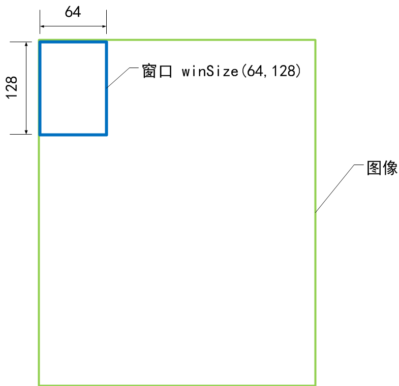
下面我们就把注意力放在前面的构造函数的参数上面吧,这里有几个重要的参数要研究下:winSize(64,128), blockSize(16,16), blockStride(8,8), cellSize(8,8), nbins(9)。上面这些都是HOGDescriptor的成员变量,括号里的数值是它们的默认值,它们反应了HOG描述子的参数。这里做了几个示意图来表示它们的含义。
窗口大小 winSize
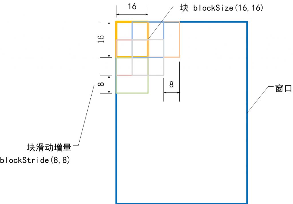
块大小 blockSize
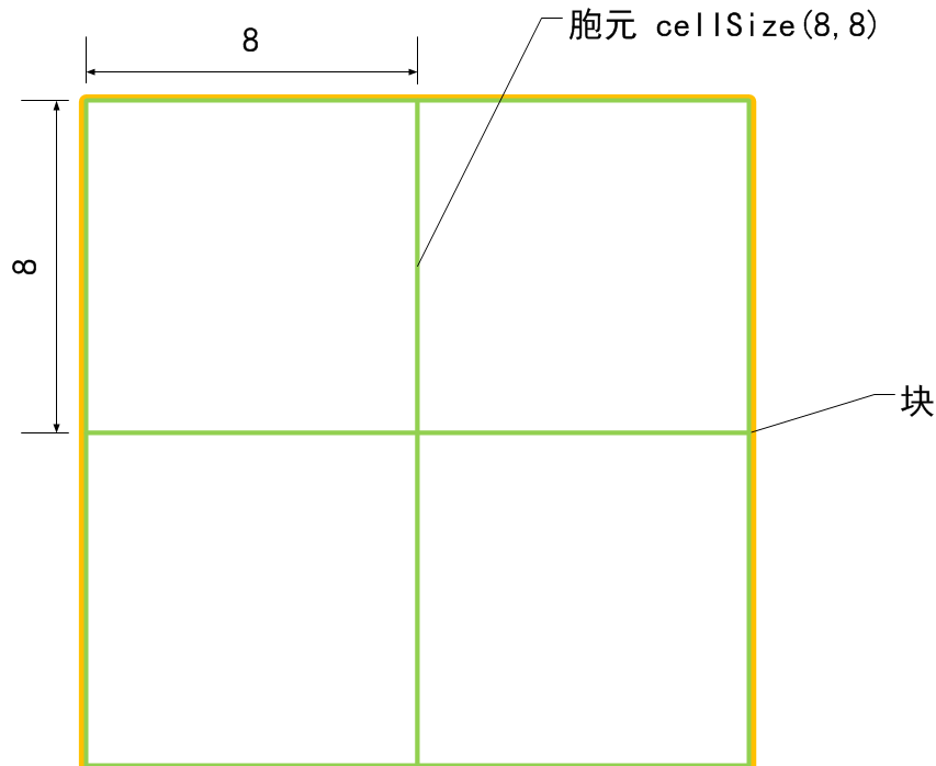
胞元大小 cellSize
梯度方向数 nbins
nBins表示在一个胞元(cell)中统计梯度的方向数目,例如nBins=9时,在一个胞元内统计9个方向的梯度直方图,每个方向为180/9=20度。
HOG描述子维度
在确定了上述的参数后,我们就可以计算出一个HOG描述子的维度了。OpenCV中的HOG源代码是按照下面的式子计算出描述子的维度的。
- size_t HOGDescriptor::getDescriptorSize() const
- {
- CV_Assert(blockSize.width % cellSize.width == 0 &&
- blockSize.height % cellSize.height == 0);
- CV_Assert((winSize.width - blockSize.width) % blockStride.width == 0 &&
- (winSize.height - blockSize.height) % blockStride.height == 0 );
- return (size_t)nbins*
- (blockSize.width/cellSize.width)*
- (blockSize.height/cellSize.height)*
- ((winSize.width - blockSize.width)/blockStride.width + 1)*
- ((winSize.height - blockSize.height)/blockStride.height + 1);
- }
- Histograms of Oriented Gradients (HOG)理解和源码
- Histograms of Oriented Gradients (HOG)理解和源码
- Histograms of Oriented Gradients (HOG)理解和源码
- Histograms of Oriented Gradients (HOG)理解和源码
- Histograms of Oriented Gradients (HOG)理解和源码
- Histograms of Oriented Gradients (HOG)理解和源码
- Histograms of Oriented Gradients (HOG)理解和源码
- Histograms of Oriented Gradients (HOG)理解和源码
- (转载)Histograms of Oriented Gradients (HOG)理解
- 【原理】Histograms of Oriented Gradients (HOG)理解
- Histograms of Oriented Gradients (HOG)理解
- Histograms of Oriented Gradients (HOG)理解
- Histograms of Oriented Gradients (HOG)描述子理解
- HOG特征 (Histograms of Oriented Gradients)
- Histograms of Oriented Gradients
- HIstograms of Oriented Gradients
- 方向梯度直方图HOG:Histograms of Oriented Gradients 及matlab源码
- Histograms of Oriented Gradients (HOG)特征 MATLAB 计算
- NSoperation的疑惑
- js中encode、decode的应用说明
- MySQL查询优化--数据类型与效率
- missing break in switch.
- ANT及build.xml文档编写
- Histograms of Oriented Gradients (HOG)理解和源码
- javascript处理json
- DM368 Uboot
- IdentityServlet
- TimesTen在linux下的安装
- mysql中having语句与where语句的用法与区别
- Android NDK之----- C调用Java [GetMethodID方法的使用]
- Eclipse各种小图标含义
- 查询之order by,group by和having的使用