Tamura texture features

 

 

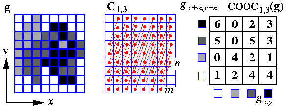
上图是灰度共生矩阵的原理图。

原理可以详细阅读有关论文，这里有详细介绍：查看链接

基于人类对纹理的视觉感知的心理学的研究，Tamura等人提出了纹理特征的表达[14]。Tamura纹理特征的六个分量对应于心理学角度上纹理特征的六种属性，分别是粗糙度（coarseness）、对比度（contrast）、方向度（directionality）、 线像度（linelikeness）、规整度（regularity）和粗略度（roughness）。其中，前三个分量对于图像检索尤其重要

Tamura's Texture Features

Today's CBIR systems use in most cases the set of six visual features, namely,

• coarseness,
• contrast,
• directionality,
• linelikeness,
• regularity,
• roughness

selected by Tamura, Mori, and Yamawaki (Tamura e.a., 1977, Castelli & Bergman, 2002) on the basis of psychological experiments.

Coarseness relates to distances of notable spatial variations of grey levels, that is, implicitly, to the size of the primitive elements (texels) forming the texture. The proposed computational procedure accounts for differences between the average signals for the non-overlapping windows of different size:

1. At each pixel (x,y), compute six averages for the windows of size 2^k × 2^k, k=0,1,...,5, around the pixel.
2. At each pixel, compute absolute differencesE_k(x,y) between the pairs of nonoverlapping averages in the horizontal and vertical directions.
3. At each pixel, find the value of k that maximises the difference E_k(x,y) in either direction and set the best size S_best(x,y)=2^k.
4. Compute the coarseness feature F_crs by averaging S_best(x,y) over the entire image.

Instead of the average of S_best(x,y, an improved coarseness feature to deal with textures having multiple coarseness properties is a histogram characterising the whole distribution of the best sizes over the image (Castelli & Bergman, 2002).

Contrast measures how grey levels q; q = 0, 1, ..., q_max, vary in the image g and to what extent their distribution is biased to black or white. The second-order and normalised fourth-order central moments of the grey level histogram (empirical probability distribution), that is, the variance, σ², and kurtosis, α₄, are used to define the contrast:  where  and m is the mean grey level, i.e. the first order moment of the grey level probability distribution. The value n=0.25 is recommended as the best for discriminating the textures.

Degree of directionality is measured using the frequency distribution of oriented local edges against their directional angles. The edge strength e(x,y) and the directional angle a(x,y) are computed using the Sobel edge detector approximating the pixel-wise x- and y-derivatives of the image:

e(x,y) = 0.5(|Δ_x(x,y)| + |Δ_y(x,y)| )a(x,y) = tan^-1(Δ_y(x,y) / Δ_x(x,y))

where Δ_x(x,y) and Δ_y(x,y) are the horizontal and vertical grey level differences between the neighbouring pixels, respectively. The differences are measured using the following 3 × 3 moving window operators:

−101   1  1  1−101   0  0  0−101 −1−1−1

A histogram H_dir(a) of quantised direction values a is constructed by counting numbers of the edge pixels with the corresponding directional angles and the edge strength greater than a predefined threshold. The histogram is relatively uniform for images without strong orientation and exhibits peaks for highly directional images. The degree of directionality relates to the sharpness of the peaks: 

where n_p is the number of peaks, a_p is the position of the pth peak, w_p is the range of the angles attributed to the pth peak (that is, the range between valleys around the peak), r denotes a normalising factor related to quantising levels of the angles a, and a is the quantised directional angle (cyclically in modulo 180^o).

Three other features are highly correlated with the above three features and do not add much to the effectiveness of the texture description. The linelikeness feature F_lin is defined as an average coincidence of the edge directions (more precisely, coded directional angles) that co-occurred in the pairs of pixels separated by a distance d along the edge direction in every pixel. The edge strength is expected to be greater than a given threshold eliminating trivial "weak" edges. The coincidence is measured by the cosine of difference between the angles, so that the co-occurrences in the same direction are measured by +1 and those in the perpendicular directions by -1.

The regularity feature is defined as F_reg=1-r(s_crs+s_con+s_dir + s_lin) where r is a normalising factor and each s_... means the standard deviation of the corresponding feature F_... in each subimage the texture is partitioned into. The roughness feature is given by simply summing the coarseness and contrast measures: F_rgh=F_crs+F_con

In the most cases, only the first three Tamura's features are used for the CBIR. These features capture the high-level perceptual attributes of a texture well and are useful for image browsing. However, they are not very effective for finer texture discrimination (Castelli & Bergman, 2002).