Sparse Autoencoder3-Gradient checking and advanced optimization

来源：互联网发布：欧洲哪里最好玩知乎编辑：程序博客网时间：2024/06/03 03:35

原文：http://deeplearning.stanford.edu/wiki/index.php/Gradient_checking_and_advanced_optimization

Backpropagation is a notoriously difficult algorithm to debug and get right, especially since many subtly buggy implementations of it—for example, one that has an off-by-one error in the indices and that thus only trains some of the layers of weights, or an implementation that omits the bias term—will manage to learn something that can look surprisingly reasonable (while performing less well than a correct implementation). Thus, even with a buggy implementation, it may not at all be apparent that anything is amiss. In this section, we describe a method for numerically checking the derivatives computed by your code to make sure that your implementation is correct. Carrying out the derivative checking procedure described here will significantly increase your confidence in the correctness of your code.

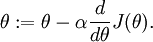
Suppose we want to minimize $\textstyle J(\theta)$ as a function of $\textstyle \theta$ . For this example, suppose $\textstyle J : \Re \mapsto \Re$ , so that $\textstyle \theta \in \Re$ . In this 1-dimensional case, one iteration of gradient descent is given by

$\begin{align}\theta := \theta - \alpha \frac{d}{d\theta}J(\theta).\end{align}$

Suppose also that we have implemented some function $\textstyle g(\theta)$ that purportedly computes $\textstyle \frac{d}{d\theta}J(\theta)$ , so that we implement gradient descent using the update 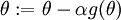$\textstyle \theta := \theta - \alpha g(\theta)$ . How can we check if our implementation of $\textstyle g$ is correct?

Recall the mathematical definition of the derivative as

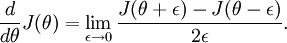
$\begin{align}\frac{d}{d\theta}J(\theta) = \lim_{\epsilon \rightarrow 0}\frac{J(\theta+ \epsilon) - J(\theta-\epsilon)}{2 \epsilon}.\end{align}$

Thus, at any specific value of $\textstyle \theta$ , we can numerically approximate the derivative as follows:

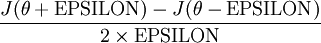
$\begin{align}\frac{J(\theta+{\rm EPSILON}) - J(\theta-{\rm EPSILON})}{2 \times {\rm EPSILON}}\end{align}$

In practice, we set $EPSILON$ to a small constant, say around $\textstyle 10^{-4}$ . (There's a large range of values of $EPSILON$ that should work well, but we don't set $EPSILON$ to be "extremely" small, say $\textstyle 10^{-20}$ , as that would lead to numerical roundoff errors.)

Thus, given a function $\textstyle g(\theta)$ that is supposedly computing $\textstyle \frac{d}{d\theta}J(\theta)$ , we can now numerically verify its correctness by checking that

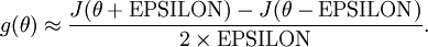
$\begin{align}g(\theta) \approx\frac{J(\theta+{\rm EPSILON}) - J(\theta-{\rm EPSILON})}{2 \times {\rm EPSILON}}.\end{align}$

The degree to which these two values should approximate each other will depend on the details of $\textstyle J$ . But assuming 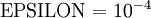$\textstyle {\rm EPSILON} = 10^{-4}$ , you'll usually find that the left- and right-hand sides of the above will agree to at least 4 significant digits (and often many more).

Now, consider the case where $\textstyle \theta \in \Re^n$ is a vector rather than a single real number (so that we have $\textstyle n$ parameters that we want to learn), and $\textstyle J: \Re^n \mapsto \Re$ . In our neural network example we used " $\textstyle J(W,b)$ ," but one can imagine "unrolling" the parameters $\textstyle W,b$ into a long vector $\textstyle \theta$ . We now generalize our derivative checking procedure to the case where $\textstyle \theta$ may be a vector.

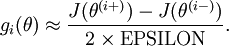
Suppose we have a function $\textstyle g_i(\theta)$ that purportedly computes $\textstyle \frac{\partial}{\partial \theta_i} J(\theta)$ ; we'd like to check if $\textstyle g_i$ is outputting correct derivative values. Let $\textstyle \theta^{(i+)} = \theta +{\rm EPSILON} \times \vec{e}_i$ , where

$\begin{align}\vec{e}_i = \begin{bmatrix}0 \\ 0 \\ \vdots \\ 1 \\ \vdots \\ 0\end{bmatrix}\end{align}$

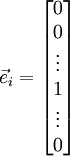
is the $\textstyle i$ -th basis vector (a vector of the same dimension as $\textstyle \theta$ , with a "1" in the $\textstyle i$ -th position and "0"s everywhere else). So, $\textstyle \theta^{(i+)}$ is the same as $\textstyle \theta$ , except its $\textstyle i$ -th element has been incremented by $EPSILON$ . Similarly, let $\textstyle \theta^{(i-)} = \theta - {\rm EPSILON} \times \vec{e}_i$ be the corresponding vector with the $\textstyle i$ -th element decreased by $EPSILON$ . We can now numerically verify $\textstyle g_i(\theta)$ 's correctness by checking, for each $\textstyle i$ , that:

$\begin{align}g_i(\theta) \approx\frac{J(\theta^{(i+)}) - J(\theta^{(i-)})}{2 \times {\rm EPSILON}}.\end{align}$

When implementing backpropagation to train a neural network, in a correct implementation we will have that

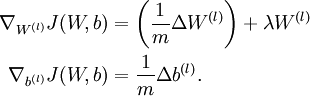
$\begin{align}\nabla_{W^{(l)}} J(W,b) &= \left( \frac{1}{m} \Delta W^{(l)} \right) + \lambda W^{(l)} \\\nabla_{b^{(l)}} J(W,b) &= \frac{1}{m} \Delta b^{(l)}.\end{align}$

This result shows that the final block of psuedo-code in Backpropagation Algorithm is indeed implementing gradient descent. To make sure your implementation of gradient descent is correct, it is usually very helpful to use the method described above to numerically compute the derivatives of $\textstyle J(W,b)$ , and thereby verify that your computations of 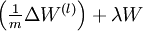$\textstyle \left(\frac{1}{m}\Delta W^{(l)} \right) + \lambda W$ and $\textstyle \frac{1}{m}\Delta b^{(l)}$ are indeed giving the derivatives you want.

Finally, so far our discussion has centered on using gradient descent to minimize $\textstyle J(\theta)$ . If you have implemented a function that computes $\textstyle J(\theta)$ and $\textstyle \nabla_\theta J(\theta)$ , it turns out there are more sophisticated algorithms than gradient descent for trying to minimize $\textstyle J(\theta)$ . For example, one can envision an algorithm that uses gradient descent, but automatically tunes the learning rate $\textstyle \alpha$ so as to try to use a step-size that causes $\textstyle \theta$ to approach a local optimum as quickly as possible. There are other algorithms that are even more sophisticated than this; for example, there are algorithms that try to find an approximation to the Hessian matrix, so that it can take more rapid steps towards a local optimum (similar to Newton's method). A full discussion of these algorithms is beyond the scope of these notes, but one example is the L-BFGS algorithm. (Another example is the conjugate gradient algorithm.) You will use one of these algorithms in the programming exercise. The main thing you need to provide to these advanced optimization algorithms is that for any $\textstyle \theta$ , you have to be able to compute $\textstyle J(\theta)$ and $\textstyle \nabla_\theta J(\theta)$ . These optimization algorithms will then do their own internal tuning of the learning rate/step-size $\textstyle \alpha$ (and compute its own approximation to the Hessian, etc.) to automatically search for a value of $\textstyle \theta$ that minimizes $\textstyle J(\theta)$ . Algorithms such as L-BFGS and conjugate gradient can often be much faster than gradient descent.