机器学习-线性回归以及MATLAB octave实现

来源：互联网发布：广州数控980ta怎么编程编辑：程序博客网时间：2024/06/06 09:38

参考资料：

斯坦福大学公开课：机器学习课程 [第2集] 监督学习应用.梯度下降

http://v.163.com/movie/2008/1/B/O/M6SGF6VB4_M6SGHJ9BO.html

Matlab实现线性回归和逻辑回归: Linear Regression & Logistic Regression

http://blog.csdn.net/abcjennifer/article/details/7732417

octave入门教程

http://wenku.baidu.com/view/22f5bb10cc7931b765ce1588.html

关于非线性优化fminbnd函数的说明（仅供新手参考）（也可作为fmincon函数的参考）

http://hi.baidu.com/maodoulovexixi/item/4205be1c11fbce6d3e87ce39

http://www.docin.com/p-214776767.html

由于是刚开始接触ML和MATLAB，所以记录一些比较简单的笔记。

个人实验中未使用MATLAB，而是使用了Octave作为替代，区别只是把函数结束的end改成endfunction即可，其他部分和matlab保持一致。

文中主要框架内容参考 http://blog.csdn.net/abcjennifer/article/details/7732417

第一部分：基本模型

在解决拟合问题的解决之前，我们首先回忆一下线性回归基本模型。

设待拟合参数 θ_n*1 和输入参数[ x_m*n, y_m*1] 。

对于各类拟合我们都要根据梯度下降的算法，给出两部分：

① cost function（指出真实值y与拟合值h<hypothesis>之间的距离）：给出cost function 的表达式，每次迭代保证cost function的量减小；给出梯度gradient，即cost function对每一个参数θ的求导结果。

function [ jVal,gradient ] = costFunction ( theta )

② Gradient_descent（主函数）：用来运行梯度下降算法，调用上面的cost function进行不断迭代，直到最大迭代次数达到给定标准或者cost function返回值不再减小。

function [optTheta,functionVal,exitFlag]=Gradient_descent( )

线性回归：拟合方程为h_θ(x)=θ₀x₀+θ₁x₁+…+θ_nx_n，当然也可以有x_n的幂次方作为线性回归项（如），这与普通意义上的线性不同，而是类似多项式的概念。

其cost function 为：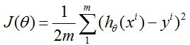

第二部分：Y=θ₀+θ₁X₁型---线性回归（直线拟合）

在Matlab 线性拟合 & 非线性拟合中我们已经讲过如何用matlab自带函数fit进行直线和曲线的拟合，非常实用。而这里我们是进行ML课程的学习，因此研究如何利用前面讲到的梯度下降法（gradient descent）进行拟合。

cost function：

[cpp] view plaincopy
function [ jVal,gradient ] = costFunction2( theta )  
%COSTFUNCTION2 Summary of this function goes here  
%   linear regression -> y=theta0 + theta1*x  
%   parameter: x:m*n  theta:n*1   y:m*1   (m=4,n=1)  
%     
  
%Data  
x=[1;2;3;4];  
y=[1.1;2.2;2.7;3.8];  
m=size(x,1);  
  
hypothesis = h_func(x,theta);  
delta = hypothesis - y;  
jVal=sum(delta.^2);  
  
gradient(1)=sum(delta)/m;  
gradient(2)=sum(delta.*x)/m;  
  
end  

其中，h_func是hypothesis的结果：

[cpp] view plaincopy
function [res] = h_func(inputx,theta)  
%H_FUNC Summary of this function goes here  
%   Detailed explanation goes here  
  
  
%cost function 2  
res= theta(1)+theta(2)*inputx;  
end  

Gradient_descent：

[cpp] view plaincopy
function [optTheta,functionVal,exitFlag]=Gradient_descent( )  
%GRADIENT_DESCENT Summary of this function goes here  
%   Detailed explanation goes here  
  
  options = optimset('GradObj','on','MaxIter',100);  
  initialTheta = zeros(2,1);  
  [optTheta,functionVal,exitFlag] = fminunc(@costFunction2,initialTheta,options);  
  
end  

result：

[cpp] view plaincopy
>> [optTheta,functionVal,exitFlag] = Gradient_descent()  
  
Local minimum found.  
  
Optimization completed because the size of the gradient is less than  
the default value of the function tolerance.  
  
<stopping criteria details>  
  
optTheta =  
  
    0.3000  
    0.8600  
  
functionVal =  
  
    0.0720  
  
exitFlag =  
  
     1

即得y=0.3+0.86x;

验证：

[cpp] view plaincopy
function [ parameter ] = checkcostfunc(  )  
%CHECKC2 Summary of this function goes here  
%   check if the cost function works well  
%   check with the matlab fit function as standard  
  
%check cost function 2  
x=[1;2;3;4];  
y=[1.1;2.2;2.7;3.8];  
  
EXPR= {'x','1'};  
p=fittype(EXPR);  
parameter=fit(x,y,p);  
  
end  

运行结果：

[cpp] view plaincopy
>> checkcostfunc()  
  
ans =   
  
     Linear model:  
     ans(x) = a*x + b  
     Coefficients (with 95% confidence bounds):  
       a =        0.86  (0.4949, 1.225)  
       b =         0.3  (-0.6998, 1.3)  

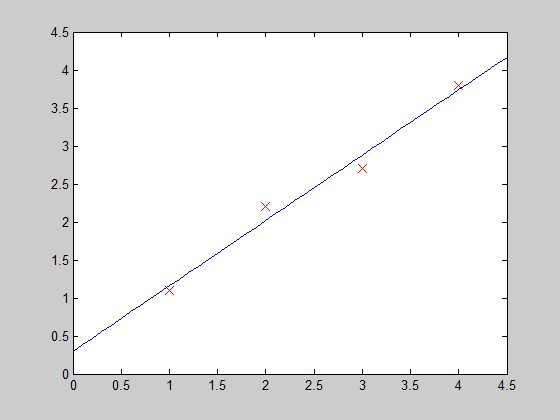
和我们的结果一样。下面画图：

[cpp] view plaincopy
function PlotFunc( xstart,xend )  
%PLOTFUNC Summary of this function goes here  
%   draw original data and the fitted   
  
  
  
%===================cost function 2====linear regression  
%original data  
x1=[1;2;3;4];  
y1=[1.1;2.2;2.7;3.8];  
%plot(x1,y1,'ro-','MarkerSize',10);  
plot(x1,y1,'rx','MarkerSize',10);  
hold on;  
  
%fitted line - 拟合曲线  
x_co=xstart:0.1:xend;  
y_co=0.3+0.86*x_co;  
%plot(x_co,y_co,'g');  
plot(x_co,y_co);  
  
hold off;  
end  

注解：

1 single training example公式

More than one training example:

θ：θ(i)-=gradient(i),其中gradient(i)是J(θ)对θi求导的函数式,此处令α=1/m，并且gradient(1)在matlab程序中实际对应x(0),而x(0)=1，把代入上面的公式可以得到gradient(1)=sum(delta)/m;

注解2

options = optimset('GradObj','on','MaxIter',100);
initialTheta = zeros(2,1);
[optTheta,functionVal,exitFlag] = fminunc(@costFunction2,initialTheta,options);

初学matlab优化，迭代中止后，经常一头雾水。参看帮助后仍似懂非懂。下面关于fminbnd函数的说明（也可作为fmincon函数的参考）对于新手也许会有帮助，不当之处请指正。
目标函数fun:
   需要最小化的目标函数。fun函数需要输入标量参数x，返回x处的目标函数标量值f。可以将fun函数指定为命令行，如
         x = fminbnd(inline('sin(x*x)'),x0)
同样，fun参数可以是一个包含函数名的字符串。对应的函数可以是M文件、内部函数或MEX文件。若fun='myfun'，则M文件函数myfun.m必须有下面的形式：
         function f = myfun(x)
         f = ...          %计算x处的函数值。
若fun函数的梯度可以算得，且options.GradObj设为'on'（用下式设定）,
         options = optimset('GradObj','on')
则fun函数必须返回解x处的梯度向量g到第二个输出变量中去。注意，当被调用的fun函数只需要一个输出变量时（如算法只需要目标函数的值而不需要其梯度值时），可以通过核对nargout的值来避免计算梯度值。
function [f,g] = myfun(x)
f = ...       %计算x处得函数值。
if nargout > 1 %调用fun函数并要求有两个输出变量。
g = ...    %计算x处的梯度值。
end