Exercise 4: Logistic Regression and Newton's Method

来源：互联网发布：java链表原理编辑：程序博客网时间：2024/04/30 17:19

In this exercise, you will use Newton's Method to implement logistic regression on a classification problem.

Data

For this exercise, suppose that a high school has a dataset representing 40 students who were admitted to college and 40 students who were not admitted. Each $(x^{(i)}, y^{(i)})$ training example contains a student's score on two standardized exams and a label of whether the student was admitted.

Your task is to build a binary classification model that estimates college admission chances based on a student's scores on two exams. In your training data,

a. The first column of your x array represents all Test 1 scores, and the second column represents all Test 2 scores.

b. The y vector uses '1' to label a student who was admitted and '0' to label a student who was not admitted.

Plot the data

Load the data for the training examples into your program and add the intercept term into your x matrix.

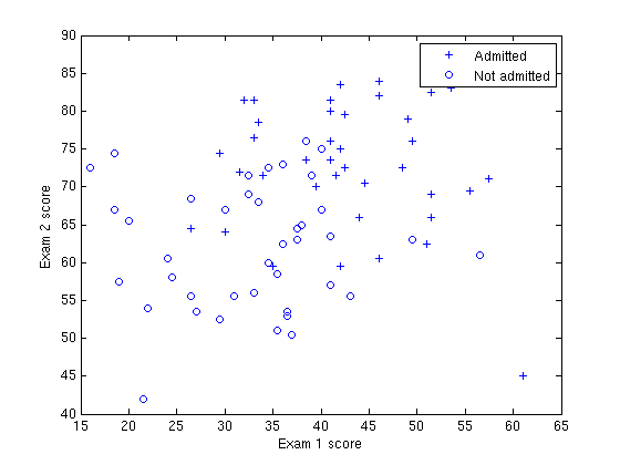
Before beginning Newton's Method, we will first plot the data using different symbols to represent the two classes. In Matlab/Octave, you can separate the positive class and the negative class using the find command:

% find returns the indices of the% rows meeting the specified conditionpos = find(y == 1); neg = find(y == 0);% Assume the features are in the 2nd and 3rd% columns of xplot(x(pos, 2), x(pos,3), '+'); hold onplot(x(neg, 2), x(neg, 3), 'o')

Your plot should look like the following:

Newton's Method

Recall that in logistic regression, the hypothesis function is

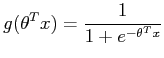
$\displaystyle h_{\theta}(x)$ $\textstyle =$ $\displaystyle g(\theta^{T}x)=\frac{{1}}{1+e^{-\theta^{T}x}}$ $\textstyle =$ $\displaystyle P(y=1\vert x;\theta)$

In our example, the hypothesis is interpreted as the probability that a driver will be accident-free, given the values of the features in x.

Matlab/Octave does not have a library function for the sigmoid, so you will have to define it yourself. The easiest way to do this is through an inline expression:

g = inline('1.0 ./ (1.0 + exp(-z))'); % Usage: To find the value of the sigmoid % evaluated at 2, call g(2)

The cost function $J(\theta)$ is defined as

$\begin{displaymath}J(\theta)=\frac{{1}}{m}\sum_{i=1}^{m}\left[-y^{(i)}\log(h_......(1-y^{(i)})\log(1-h_{\theta}(x^{(i)}))\right] \nonumber\par\end{displaymath}$

Our goal is to use Newton's method to minimize this function. Recall that the update rule for Newton's method is

$\begin{displaymath}\theta^{(t+1)}=\theta^{(t)}-H^{-1}\nabla_{\theta}J \nonumber\end{displaymath}$

In logistic regression, the gradient and the Hessian are

$\begin{displaymath}\nabla_{\theta}J = \frac{1}{m}\sum_{i=1}^{m}(h_{\theta}(x^{(i)})-y^{(i)})x^{(i)} \nonumber \nonumber\end{displaymath}$

$\begin{displaymath}H & = & \frac{1}{m}\sum_{i=1}^{m}\left[h_{\theta}(x^{(i)})\l......^{(i)})\right)x^{(i)}\left(x^{(i)}\right)^{T}\right] \nonumber\end{displaymath}$

Note that the formulas presented above are the vectorized versions. Specifically, this means that $x^{(i)} \in R^{n+1}$ , $x^{(i)}\left(x^{(i)}\right)^{T}\in R^{(n+1) \times (n+1)}$ , while $h_{\theta}(x^{(i)})$ and $y^{(i)}$ are scalars.

Implementation

Now, implement Newton's Method in your program, starting with the initial value of $\theta = \vec{0}$ . To determine how many iterations to use, calculate $J(\theta)$ for each iteration and plot your results as you did in Exercise 2. As mentioned in the lecture videos, Newton's method often converges in 5-15 iterations. If you find yourself using far more iterations, you should check for errors in your implementation.

After convergence, use your values of theta to find the decision boundary in the classification problem. The decision boundary is defined as the line where

$\begin{displaymath}P(y=1\vert x; \theta) = g(\theta^T x) = 0.5\end{displaymath}$

which corresponds to

$\begin{displaymath}\theta^T x = 0\end{displaymath}$

Plotting the decision boundary is equivalent to plotting the $\theta^T x = 0$ line. When you are finished, your plot should appear like the figure below.

Questions

Finally, record your answers to these questions.

1. What values of $\theta$ did you get? How many iterations were required for convergence?

2. What is the probability that a student with a score of 20 on Exam 1 and a score of 80 on Exam 2 will not be admitted?

Solutions

After you have completed the exercises above, please refer to the solutions below and check that your implementation and your answers are correct. In a case where your implementation does not result in the same parameters/phenomena as described below, debug your solution until you manage to replicate the same effect as our implementation.
Newton's Method

1. Your final values of theta should be

$\displaystyle \theta_0$ $\textstyle =$ $\displaystyle -16.38$ $\displaystyle \theta_1$ $\textstyle =$ $\displaystyle 0.1483$ $\displaystyle \theta_2$ $\textstyle =$ $\displaystyle 0.1589$

Plot. Your plot of the cost function should look similar to the picture below:

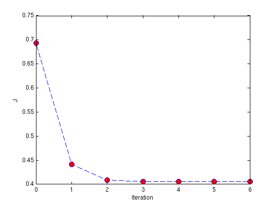
From this plot, you can infer that Newton's Method has converged by around 5 iterations. In fact, by looking at a printout of the values of J, you will see that J changes by less than $10^{-7}$ between the 4th and 5th iterations. Recall that in the previous two exercises, gradient descent took hundreds or even thousands of iterations to converge. Newton's Method is much faster in comparison.

2. The probability that a student with a score of 20 on Exam 1 and 80 on Exam 2 will not be admitted to college is 0.668.