UFLDL Tutorial_Building Deep Networks for Classification

Self-Taught Learning to Deep Networks

In the previous section, you used an autoencoder to learn features that were then fed as input to a softmax or logistic regression classifier. In that method, the features were learned using only unlabeled data. In this section, we describe how you can fine-tune and further improve the learned features using labeled data. When you have a large amount of labeled training data, this can significantly improve your classifier's performance.

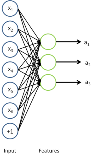
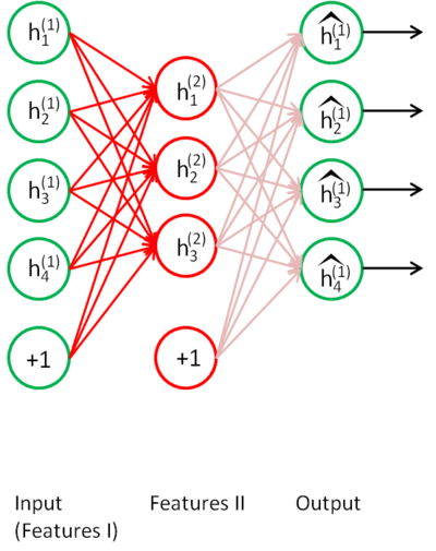
In self-taught learning, we first trained a sparse autoencoder on the unlabeled data. Then, given a new example , we used the hidden layer to extract features . This is illustrated in the following diagram:

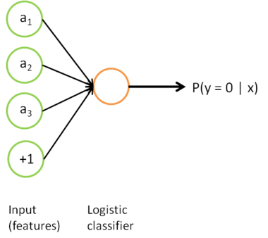
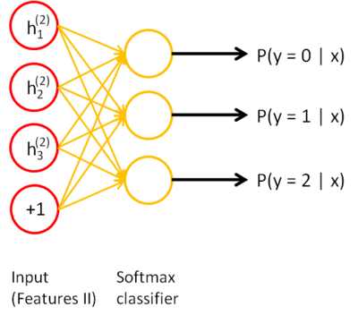
We are interested in solving a classification task, where our goal is to predict labels . We have a labeled training set  of  labeled examples. We showed previously that we can replace the original features with features  computed by the sparse autoencoder (the "replacement" representation). This gives us a training set . Finally, we train a logistic classifier to map from the features  to the classification label . To illustrate this step, similar to our earlier notes, we can draw our logistic regression unit (shown in orange) as follows:

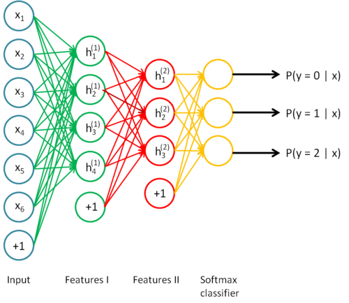
Now, consider the overall classifier (i.e., the input-output mapping) that we have learned using this method. In particular, let us examine the function that our classifier uses to map from from a new test example  to a new prediction p(y = 1 | x). We can draw a representation of this function by putting together the two pictures from above. In particular, the final classifier looks like this:

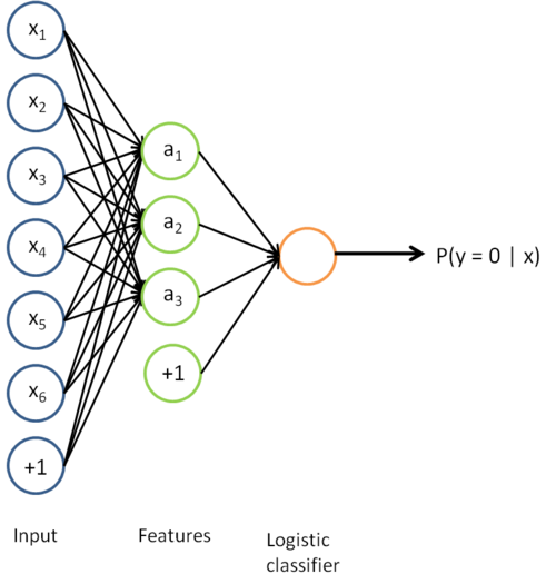
The parameters of this model were trained in two stages: The first layer of weights  mapping from the input  to the hidden unit activations  were trained as part of the sparse autoencoder training process. The second layer of weights  mapping from the activations  to the output  was trained using logistic regression (or softmax regression).

But the form of our overall/final classifier is clearly just a whole big neural network. So, having trained up an initial set of parameters for our model (training the first layer using an autoencoder, and the second layer via logistic/softmax regression), we can further modify all the parameters in our model to try to further reduce the training error. In particular, we can fine-tunethe parameters, meaning perform gradient descent (or use L-BFGS) from the current setting of the parameters to try to reduce the training error on our labeled training set .

When fine-tuning is used, sometimes the original unsupervised feature learning steps (i.e., training the autoencoder and the logistic classifier) are called pre-training. The effect of fine-tuning is that the labeled data can be used to modify the weightsW⁽¹⁾ as well, so that adjustments can be made to the features a extracted by the layer of hidden units.

So far, we have described this process assuming that you used the "replacement" representation, where the training examples seen by the logistic classifier are of the form (a⁽ⁱ⁾,y⁽ⁱ⁾), rather than the "concatenation" representation, where the examples are of the form ((x⁽ⁱ⁾,a⁽ⁱ⁾),y⁽ⁱ⁾). It is also possible to perform fine-tuning too using the "concatenation" representation. (This corresponds to a neural network where the input units x_i also feed directly to the logistic classifier in the output layer. You can draw this using a slightly different type of neural network diagram than the ones we have seen so far; in particular, you would have edges that go directly from the first layer input nodes to the third layer output node, "skipping over" the hidden layer.) However, so long as we are using finetuning, usually the "concatenation" representation has little advantage over the "replacement" representation. Thus, if we are using fine-tuning usually we will do so with a network built using the replacement representation. (If you are not using fine-tuning however, then sometimes the concatenation representation can give much better performance.)

When should we use fine-tuning? It is typically used only if you have a large labeled training set; in this setting, fine-tuning can significantly improve the performance of your classifier. However, if you have a large unlabeled dataset (for unsupervised feature learning/pre-training) and only a relatively small labeled training set, then fine-tuning is significantly less likely to help.

Deep Networks: Overview

Contents

 [hide]

• 1 Overview
• 2 Advantages of deep networks
• 3 Difficulty of training deep architectures
  • 3.1 Availability of data
  • 3.2 Local optima
  • 3.3 Diffusion of gradients
• 4 Greedy layer-wise training
  • 4.1 Availability of data
  • 4.2 Better local optima

Overview

In the previous sections, you constructed a 3-layer neural network comprising an input, hidden and output layer. While fairly effective for MNIST, this 3-layer model is a fairly shallow network; by this, we mean that the features (hidden layer activationsa⁽²⁾) are computed using only "one layer" of computation (the hidden layer).

In this section, we begin to discuss deep neural networks, meaning ones in which we have multiple hidden layers; this will allow us to compute much more complex features of the input. Because each hidden layer computes a non-linear transformation of the previous layer, a deep network can have significantly greater representational power (i.e., can learn significantly more complex functions) than a shallow one.

Note that when training a deep network, it is important to use a non-linear activation function  in each hidden layer. This is because multiple layers of linear functions would itself compute only a linear function of the input (i.e., composing multiple linear functions together results in just another linear function), and thus be no more expressive than using just a single layer of hidden units.

Advantages of deep networks

Why do we want to use a deep network? The primary advantage is that it can compactly represent a significantly larger set of fuctions than shallow networks. Formally, one can show that there are functions which a k-layer network can represent compactly (with a number of hidden units that is polynomial in the number of inputs), that a (k − 1)-layer network cannot represent unless it has an exponentially large number of hidden units.

To take a simple example, consider building a boolean circuit/network to compute the parity (or XOR) of n input bits. Suppose each node in the network can compute either the logical OR of its inputs (or the OR of the negation of the inputs), or compute the logical AND. If we have a network with only one input, one hidden, and one output layer, the parity function would require a number of nodes that is exponential in the input size n. If however we are allowed a deeper network, then the network/circuit size can be only polynomial in n.

By using a deep network, in the case of images, one can also start to learn part-whole decompositions. For example, the first layer might learn to group together pixels in an image in order to detect edges (as seen in the earlier exercises). The second layer might then group together edges to detect longer contours, or perhaps detect simple "parts of objects." An even deeper layer might then group together these contours or detect even more complex features.

Finally, cortical computations (in the brain) also have multiple layers of processing. For example, visual images are processed in multiple stages by the brain, by cortical area "V1", followed by cortical area "V2" (a different part of the brain), and so on.

Difficulty of training deep architectures

While the theoretical benefits of deep networks in terms of their compactness and expressive power have been appreciated for many decades, until recently researchers had little success training deep architectures.

The main learning algorithm that researchers were using was to randomly initialize the weights of a deep network, and then train it using a labeled training set  using a supervised learning objective, for example by applying gradient descent to try to drive down the training error. However, this usually did not work well. There were several reasons for this.

Availability of data

With the method described above, one relies only on labeled data for training. However, labeled data is often scarce, and thus for many problems it is difficult to get enough examples to fit the parameters of a complex model. For example, given the high degree of expressive power of deep networks, training on insufficient data would also result in overfitting.

Local optima

Training a shallow network (with 1 hidden layer) using supervised learning usually resulted in the parameters converging to reasonable values; but when we are training a deep network, this works much less well. In particular, training a neural network using supervised learning involves solving a highly non-convex optimization problem (say, minimizing the training error  as a function of the network parameters ). In a deep network, this problem turns out to be rife with bad local optima, and training with gradient descent (or methods like conjugate gradient and L-BFGS) no longer work well.

Diffusion of gradients

There is an additional technical reason, pertaining to the gradients becoming very small, that explains why gradient descent (and related algorithms like L-BFGS) do not work well on a deep networks with randomly initialized weights. Specifically, when using backpropagation to compute the derivatives, the gradients that are propagated backwards (from the output layer to the earlier layers of the network) rapidly diminish in magnitude as the depth of the network increases. As a result, the derivative of the overall cost with respect to the weights in the earlier layers is very small. Thus, when using gradient descent, the weights of the earlier layers change slowly, and the earlier layers fail to learn much. This problem is often called the "diffusion of gradients."

A closely related problem to the diffusion of gradients is that if the last few layers in a neural network have a large enough number of neurons, it may be possible for them to model the labeled data alone without the help of the earlier layers. Hence, training the entire network at once with all the layers randomly initialized ends up giving similar performance to training a shallow network (the last few layers) on corrupted input (the result of the processing done by the earlier layers).

Greedy layer-wise training

How can we train a deep network? One method that has seen some success is the greedy layer-wise training method. We describe this method in detail in later sections, but briefly, the main idea is to train the layers of the network one at a time, so that we first train a network with 1 hidden layer, and only after that is done, train a network with 2 hidden layers, and so on. At each step, we take the old network with k − 1 hidden layers, and add an additional k-th hidden layer (that takes as input the previous hidden layer k − 1 that we had just trained). Training can either be supervised (say, with classification error as the objective function on each step), but more frequently it is unsupervised (as in an autoencoder; details to provided later). The weights from training the layers individually are then used to initialize the weights in the final/overall deep network, and only then is the entire architecture "fine-tuned" (i.e., trained together to optimize the labeled training set error).

The success of greedy layer-wise training has been attributed to a number of factors:

Availability of data

While labeled data can be expensive to obtain, unlabeled data is cheap and plentiful. The promise of self-taught learning is that by exploiting the massive amount of unlabeled data, we can learn much better models. By using unlabeled data to learn a good initial value for the weights in all the layers  (except for the final classification layer that maps to the outputs/predictions), our algorithm is able to learn and discover patterns from massively more amounts of data than purely supervised approaches. This often results in much better classifiers being learned.

Better local optima

After having trained the network on the unlabeled data, the weights are now starting at a better location in parameter space than if they had been randomly initialized. We can then further fine-tune the weights starting from this location. Empirically, it turns out that gradient descent from this location is much more likely to lead to a good local minimum, because the unlabeled data has already provided a significant amount of "prior" information about what patterns there are in the input data.

In the next section, we will describe the specific details of how to go about implementing greedy layer-wise training.

Stacked Autoencoders

Contents

 [hide]

• 1 Overview
• 2 Training
• 3 Concrete example
• 4 Discussion

Overview

The greedy layerwise approach for pretraining a deep network works by training each layer in turn. In this page, you will find out how autoencoders can be "stacked" in a greedy layerwise fashion for pretraining (initializing) the weights of a deep network.

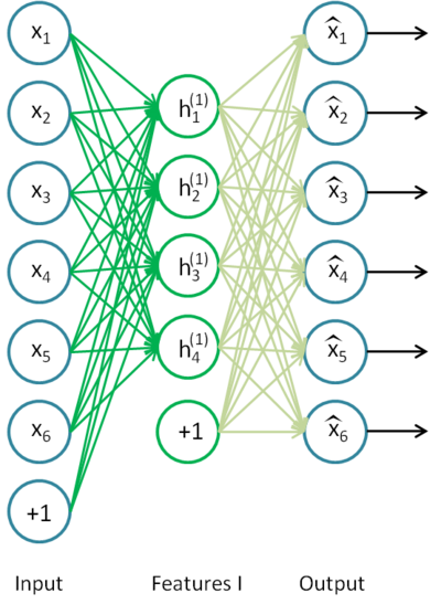
A stacked autoencoder is a neural network consisting of multiple layers of sparse autoencoders in which the outputs of each layer is wired to the inputs of the successive layer. Formally, consider a stacked autoencoder with n layers. Using notation from the autoencoder section, let W^(k,1),W^(k,2),b^(k,1),b^(k,2) denote the parameters W⁽¹⁾,W⁽²⁾,b⁽¹⁾,b⁽²⁾ for kth autoencoder. Then the encoding step for the stacked autoencoder is given by running the encoding step of each layer in forward order:

The decoding step is given by running the decoding stack of each autoencoder in reverse order:

The information of interest is contained within a⁽ⁿ⁾, which is the activation of the deepest layer of hidden units. This vector gives us a representation of the input in terms of higher-order features.

The features from the stacked autoencoder can be used for classification problems by feeding a(n) to a softmax classifier.

Training

A good way to obtain good parameters for a stacked autoencoder is to use greedy layer-wise training. To do this, first train the first layer on raw input to obtain parameters W^(1,1),W^(1,2),b^(1,1),b^(1,2). Use the first layer to transform the raw input into a vector consisting of activation of the hidden units, A. Train the second layer on this vector to obtain parametersW^(2,1),W^(2,2),b^(2,1),b^(2,2). Repeat for subsequent layers, using the output of each layer as input for the subsequent layer.

This method trains the parameters of each layer individually while freezing parameters for the remainder of the model. To produce better results, after this phase of training is complete, fine-tuning using backpropagation can be used to improve the results by tuning the parameters of all layers are changed at the same time.

If one is only interested in finetuning for the purposes of classification, the common practice is to then discard the "decoding" layers of the stacked autoencoder and link the last hidden layer a⁽ⁿ⁾ to the softmax classifier. The gradients from the (softmax) classification error will then be backpropagated into the encoding layers.

Concrete example

To give a concrete example, suppose you wished to train a stacked autoencoder with 2 hidden layers for classification of MNIST digits, as you will be doing in the next exercise.

First, you would train a sparse autoencoder on the raw inputs x^(k) to learn primary features h^(1)(k) on the raw input.

Next, you would feed the raw input into this trained sparse autoencoder, obtaining the primary feature activations h^(1)(k) for each of the inputs x^(k). You would then use these primary features as the "raw input" to another sparse autoencoder to learn secondary features h^(2)(k) on these primary features.

Following this, you would feed the primary features into the second sparse autoencoder to obtain the secondary feature activationsh^(2)(k) for each of the primary features h^(1)(k) (which correspond to the primary features of the corresponding inputs x^(k)). You would then treat these secondary features as "raw input" to a softmax classifier, training it to map secondary features to digit labels.

Finally, you would combine all three layers together to form a stacked autoencoder with 2 hidden layers and a final softmax classifier layer capable of classifying the MNIST digits as desired.

Discussion

A stacked autoencoder enjoys all the benefits of any deep network of greater expressive power.

Further, it often captures a useful "hierarchical grouping" or "part-whole decomposition" of the input. To see this, recall that an autoencoder tends to learn features that form a good representation of its input. The first layer of a stacked autoencoder tends to learn first-order features in the raw input (such as edges in an image). The second layer of a stacked autoencoder tends to learn second-order features corresponding to patterns in the appearance of first-order features (e.g., in terms of what edges tend to occur together--for example, to form contour or corner detectors). Higher layers of the stacked autoencoder tend to learn even higher-order features.

Fine-tuning Stacked AEs

Introduction

Fine tuning is a strategy that is commonly found in deep learning. As such, it can also be used to greatly improve the performance of a stacked autoencoder. From a high level perspective, fine tuning treats all layers of a stacked autoencoder as a single model, so that in one iteration, we are improving upon all the weights in the stacked autoencoder.

General Strategy

Fortunately, we already have all the tools necessary to implement fine tuning for stacked autoencoders! In order to compute the gradients for all the layers of the stacked autoencoder in each iteration, we use the Backpropagation Algorithm, as discussed in the sparse autoencoder section. As the backpropagation algorithm can be extended to apply for an arbitrary number of layers, we can actually use this algorithm on a stacked autoencoder of arbitrary depth.

Finetuning with Backpropagation

For your convenience, the summary of the backpropagation algorithm using element wise notation is below:

1. Perform a feedforward pass, computing the activations for layers , , up to the output layer , using the equations defining the forward propagation steps.

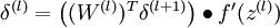
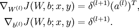
2. For the output layer (layer ), set

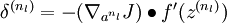
(When using softmax regression, the softmax layer has 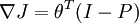 where I is the input labels and P is the vector of conditional probabilities.)

3. For 

Set

4. Compute the desired partial derivatives:

Note: While one could consider the softmax classifier as an additional layer, the derivation above does not. Specifically, we consider the "last layer" of the network to be the features that goes into the softmax classifier. Therefore, the derivatives (in Step 2) are computed using 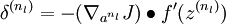, where .

Exercise: Implement deep networks for digit classification

Contents

 [hide]

• 1 Overview
• 2 Dependencies
• 3 Step 0: Initialize constants and parameters
• 4 Step 1: Train the data on the first stacked autoencoder
• 5 Step 2: Train the data on the second stacked autoencoder
• 6 Step 3: Train the softmax classifier on the L2 features
• 7 Step 4: Implement fine-tuning
• 8 Step 5: Test the model

Overview

In this exercise, you will use a stacked autoencoder for digit classification. This exercise is very similar to the self-taught learning exercise, in which we trained a digit classifier using a autoencoder layer followed by a softmax layer. The only difference in this exercise is that we will be using two autoencoder layers instead of one and further finetune the two layers.

The code you have already implemented will allow you to stack various layers and perform layer-wise training. However, to perform fine-tuning, you will need to implement backpropogation through both layers. We will see that fine-tuning significantly improves the model's performance.

In the file stackedae_exercise.zip, we have provided some starter code. You will need to complete the code in stackedAECost.m,stackedAEPredict.m and stackedAEExercise.m. We have also provided params2stack.m and stack2params.m which you might find helpful in constructing deep networks.

Dependencies

The following additional files are required for this exercise:

• MNIST Dataset
• Support functions for loading MNIST in Matlab
• Starter Code (stackedae_exercise.zip)

You will also need your code from the following exercises:

• Exercise:Sparse Autoencoder
• Exercise:Vectorization
• Exercise:Softmax Regression
• Exercise:Self-Taught Learning

If you have not completed the exercises listed above, we strongly suggest you complete them first.

Step 0: Initialize constants and parameters

Open stackedAEExercise.m. In this step, we set meta-parameters to the same values that were used in previous exercise, which should produce reasonable results. You may to modify the meta-parameters if you wish.

Step 1: Train the data on the first stacked autoencoder

Train the first autoencoder on the training images to obtain its parameters. This step is identical to the corresponding step in the sparse autoencoder and STL assignments, complete this part of the code so as to learn a first layer of features using yoursparseAutoencoderCost.m and minFunc.

Step 2: Train the data on the second stacked autoencoder

We first forward propagate the training set through the first autoencoder (using feedForwardAutoencoder.m that you completed inExercise:Self-Taught_Learning) to obtain hidden unit activations. These activations are then used to train the second sparse autoencoder. Since this is just an adapted application of a standard autoencoder, it should run similarly with the first. Complete this part of the code so as to learn a first layer of features using your sparseAutoencoderCost.m and minFunc.

This part of the exercise demonstrates the idea of greedy layerwise training with the same learning algorithm reapplied multiple times.

Step 3: Train the softmax classifier on the L2 features

Next, continue to forward propagate the L1 features through the second autoencoder (using feedForwardAutoencoder.m) to obtain the L2 hidden unit activations. These activations are then used to train the softmax classifier. You can either use softmaxTrain.m or directly use softmaxCost.m that you completed in Exercise:Softmax Regression to complete this part of the assignment.

Step 4: Implement fine-tuning

To implement fine tuning, we need to consider all three layers as a single model. Implement stackedAECost.m to return the cost and gradient of the model. The cost function should be as defined as the log likelihood and a gradient decay term. The gradient should be computed using back-propagation as discussed earlier. The predictions should consist of the activations of the output layer of the softmax model.

To help you check that your implementation is correct, you should also check your gradients on a synthetic small dataset. We have implemented checkStackedAECost.m to help you check your gradients. If this checks passes, you will have implemented fine-tuning correctly.

Note: When adding the weight decay term to the cost, you should regularize only the softmax weights (do not regularize the weights that compute the hidden layer activations).

Implementation Tip: It is always a good idea to implement the code modularly and check (the gradient of) each part of the code before writing the more complicated parts.

Step 5: Test the model

Finally, you will need to classify with this model; complete the code in stackedAEPredict.m to classify using the stacked autoencoder with a classification layer.

After completing these steps, running the entire script in stackedAETrain.m will perform layer-wise training of the stacked autoencoder, finetune the model, and measure its performance on the test set. If you've done all the steps correctly, you should get an accuracy of about 87.7% before finetuning and 97.6% after finetuning (for the 10-way classification problem).

Contents

• CS294A/CS294W Stacked Autoencoder Exercise
• STEP 0: Here we provide the relevant parameters values that will
• STEP 1: Load data from the MNIST database
• STEP 2: Train the first sparse autoencoder
• ---------------------- YOUR CODE HERE ---------------------------------
• STEP 2: Train the second sparse autoencoder
• ---------------------- YOUR CODE HERE ---------------------------------
• ---------------------- YOUR CODE HERE ---------------------------------
• STEP 3: Train the softmax classifier
• ---------------------- YOUR CODE HERE ---------------------------------
• STEP 5: Finetune softmax model
• ---------------------- YOUR CODE HERE ---------------------------------
• STEP 6: Test

CS294A/CS294W Stacked Autoencoder Exercise

%  Instructions%  ------------%%  This file contains code that helps you get started on the%  sstacked autoencoder exercise. You will need to complete code in%  stackedAECost.m%  You will also need to have implemented sparseAutoencoderCost.m and%  softmaxCost.m from previous exercises. You will need the initializeParameters.m%  loadMNISTImages.m, and loadMNISTLabels.m files from previous exercises.%%  For the purpose of completing the assignment, you do not need to%  change the code in this file.%%%======================================================================

STEP 0: Here we provide the relevant parameters values that will

allow your sparse autoencoder to get good filters; you do not need tochange the parameters below.

DISPLAY = true;inputSize = 28 * 28;numClasses = 10;hiddenSizeL1 = 196;    % Layer 1 Hidden SizehiddenSizeL2 = 64;    % Layer 2 Hidden SizehiddenSizeL3 = 25;sparsityParam = 0.1;   % desired average activation of the hidden units.                       % (This was denoted by the Greek alphabet rho, which looks like a lower-case "p",                       %  in the lecture notes).lambda = 3e-3;         % weight decay parameterbeta = 3;              % weight of sparsity penalty term%%======================================================================

STEP 1: Load data from the MNIST database

This loads our training data from the MNIST database files.

% Load MNIST database filestrainData = loadMNISTImages('train-images.idx3-ubyte');trainData=trainData(:,1:900);trainLabels = loadMNISTLabels('train-labels.idx1-ubyte');trainLabels=trainLabels(1:900);trainLabels(trainLabels == 0) = 10; % Remap 0 to 10 since our labels need to start from 1% figure% imshow(trainData(:,1:100));% % Load MNIST database files% trainData   = loadMNISTImages('train-images.idx3-ubyte');% trainData=trainData(:,1:1000);% mnistLabels = loadMNISTLabels('train-labels.idx1-ubyte');% mnistLabels=mnistLabels(1:1000);% mnistLabels(mnistLabels==0) = 10; % Remap 0 to 10%% testData   = loadMNISTImages('t10k-images.idx3-ubyte');% testData=testData(:,1:1000);% testLabels = loadMNISTLabels('t10k-labels.idx1-ubyte');% testLabels=testLabels(1:1000);% testLabels(testLabels==0) = 10; % Remap 0 to 10%debug% trainData=trainData(:,1:100);% trainLabels=trainLabels(1:100);%%======================================================================

STEP 2: Train the first sparse autoencoder

This trains the first sparse autoencoder on the unlabelled STL trainingimages.If you've correctly implemented sparseAutoencoderCost.m, you don't needto change anything here.Randomly initialize the parameters

sae1Theta = initializeParameters(hiddenSizeL1, inputSize);

---------------------- YOUR CODE HERE ---------------------------------

Instructions: Train the first layer sparse autoencoder, this layer has              an hidden size of "hiddenSizeL1"              You should store the optimal parameters in sae1OptTheta

addpath minFunc/;options = struct;options.Method = 'cg';options.maxIter = 300;options.display = 'on';[sae1OptTheta, cost] =  minFunc(@(p)sparseAutoencoderCost(p,...    inputSize,hiddenSizeL1,lambda,sparsityParam,beta,trainData),sae1Theta,options);%训练出第一层网络的参数save('saves/step2.mat', 'sae1OptTheta');%debugload('saves/step2.mat', 'sae1OptTheta');if DISPLAY  W1 = reshape(sae1OptTheta(1:hiddenSizeL1 * inputSize), hiddenSizeL1, inputSize);  display_network(W1');end% -------------------------------------------------------------------------%%======================================================================

 STEP 2: Train the second sparse autoencoder

This trains the second sparse autoencoder on the first autoencoderfeaturse.If you've correctly implemented sparseAutoencoderCost.m, you don't needto change anything here.

[sae1Features] = feedForwardAutoencoder(sae1OptTheta, hiddenSizeL1, ...                                        inputSize, trainData);%  Randomly initialize the parameterssae2Theta = initializeParameters(hiddenSizeL2, hiddenSizeL1);

---------------------- YOUR CODE HERE ---------------------------------

Instructions: Train the second layer sparse autoencoder, this layer has              an hidden size of "hiddenSizeL2" and an inputsize of              "hiddenSizeL1"

              You should store the optimal parameters in sae2OptTheta

[sae2OptTheta, cost] =  minFunc(@(p)sparseAutoencoderCost(p,...    hiddenSizeL1,hiddenSizeL2,lambda,sparsityParam,beta,sae1Features),sae2Theta,options);%训练出第一层网络的参数save('saves/step3.mat', 'sae2OptTheta');%figure;if DISPLAY  W11 = reshape(sae1OptTheta(1:hiddenSizeL1 * inputSize), hiddenSizeL1, inputSize);  W12 = reshape(sae2OptTheta(1:hiddenSizeL2 * hiddenSizeL1), hiddenSizeL2, hiddenSizeL1);%   display_network(W11');%   display_network((W12*sae1Features)',false,8);%   display_network(aaaa(1:900,:),8);  % TODO(zellyn): figure out how to display a 2-level network  %display_network(log(W11' ./ (1-W11')) * W12');%   W12_temp = W12(1:196,1:196);%   display_network(W12_temp');%   figure;%   display_network(W12_temp');sae1OptTheta_W1=W11;sae2OptTheta_W1=W12;% hi tornadomeet,% 关于如何显示high level feature的问题，我是这么做的：% *************************************** display_network((sae2OptTheta_W1*sae1OptTheta_W1)');% ***************************************% 其中sae2OptTheta_W1和sae1OptTheta_W1分别是第一层AE和第二层AE的trained weights% cheers! :Dend% -------------------------------------------------------------------------[sae2Features] = feedForwardAutoencoder(sae2OptTheta, hiddenSizeL2, ...                                        hiddenSizeL1, sae1Features);%%add 3rd  laysae3Theta = initializeParameters(hiddenSizeL3, hiddenSizeL2);

---------------------- YOUR CODE HERE ---------------------------------

Instructions: Train the second layer sparse autoencoder, this layer has              an hidden size of "hiddenSizeL2" and an inputsize of              "hiddenSizeL1"

              You should store the optimal parameters in sae2OptTheta

[sae3OptTheta, cost] =  minFunc(@(p)sparseAutoencoderCost(p,...    hiddenSizeL2,hiddenSizeL3,lambda,sparsityParam,beta,sae1Features),sae3Theta,options);%训练出第一层网络的参数save('saves/step4.mat', 'sae3OptTheta');%%======================================================================

STEP 3: Train the softmax classifier

This trains the sparse autoencoder on the second autoencoder features.If you've correctly implemented softmaxCost.m, you don't needto change anything here.

[sae3Features] = feedForwardAutoencoder(sae3OptTheta, hiddenSizeL3, ...                                        hiddenSizeL2, sae2Features); %display_network(sae2Features);%  Randomly initialize the parameterssaeSoftmaxTheta = 0.005 * randn(hiddenSizeL2 * numClasses, 1);

---------------------- YOUR CODE HERE ---------------------------------

Instructions: Train the softmax classifier, the classifier takes in              input of dimension "hiddenSizeL2" corresponding to the              hidden layer size of the 2nd layer.

              You should store the optimal parameters in saeSoftmaxOptTheta

NOTE: If you used softmaxTrain to complete this part of the exercise,      set saeSoftmaxOptTheta = softmaxModel.optTheta(:);

softmaxLambda = 1e-4;numClasses = 10;softoptions = struct;softoptions.maxIter = 400;softmaxModel = softmaxTrain(hiddenSizeL3,numClasses,softmaxLambda,...                            sae3Features,trainLabels,softoptions);saeSoftmaxOptTheta = softmaxModel.optTheta(:);save('saves/step5.mat', 'saeSoftmaxOptTheta');% -------------------------------------------------------------------------%%======================================================================

STEP 5: Finetune softmax model

% Implement the stackedAECost to give the combined cost of the whole model% then run this cell.% Initialize the stack using the parameters learnedstack = cell(3,1);%其中的saelOptTheta和sae20ptTheta都是包含了sparse autoencoder的重建层网络权值的stack{1}.w = reshape(sae1OptTheta(1:hiddenSizeL1*inputSize), ...                     hiddenSizeL1, inputSize);stack{1}.b = sae1OptTheta(2*hiddenSizeL1*inputSize+1:2*hiddenSizeL1*inputSize+hiddenSizeL1);stack{2}.w = reshape(sae2OptTheta(1:hiddenSizeL2*hiddenSizeL1), ...                     hiddenSizeL2, hiddenSizeL1);stack{2}.b = sae2OptTheta(2*hiddenSizeL2*hiddenSizeL1+1:2*hiddenSizeL2*hiddenSizeL1+hiddenSizeL2);stack{3}.w = reshape(sae3OptTheta(1:hiddenSizeL3*hiddenSizeL2), ...                     hiddenSizeL3, hiddenSizeL2);stack{3}.b = sae3OptTheta(2*hiddenSizeL3*hiddenSizeL2+1:2*hiddenSizeL3*hiddenSizeL2+hiddenSizeL3);% Initialize the parameters for the deep model[stackparams, netconfig] = stack2params(stack);stackedAETheta = [ saeSoftmaxOptTheta ; stackparams ];%stackedAETheta是个向量，为整个网络的参数，包括分类器那部分，且分类器那部分的参数放前面

---------------------- YOUR CODE HERE ----------------------------

Instructions: Train the deep network, hidden size here refers to the '              dimension of the input to the classifier, which corresponds              to "hiddenSizeL2".

[stackedAEOptTheta, cost] =  minFunc(@(p)stackedAECost(p,inputSize,hiddenSizeL2,...                         numClasses, netconfig,lambda, trainData, trainLabels),...                        stackedAETheta,options);%训练出第一层网络的参数save('saves/step5.mat', 'stackedAEOptTheta');figure;if DISPLAY  optStack = params2stack(stackedAEOptTheta(hiddenSizeL2*numClasses+1:end), netconfig);  W11 = optStack{1}.w;  W12 = optStack{2}.w;  % TODO(zellyn): figure out how to display a 2-level network   %display_network(log(1 ./ (1-W11')) * W12');enddisplay_network(W11');display_network((W12*W11)');[sae1Features] = feedForwardAutoencoder(optStack{1}, hiddenSizeL1, ...                                        inputSize, trainData);[sae2Features] = feedForwardAutoencoder(sae2OptTheta, hiddenSizeL2, ...                                        hiddenSizeL1, sae1Features);totalElem=size(trainFeatures,1)*size(trainFeatures,2);ave=sum(trainFeatures(:))/totalElemind=find(abs(trainFeatures)<0.1);sparseRate=numel(ind)/totalElem% -------------------------------------------------------------------------%%======================================================================

STEP 6: Test

Instructions: You will need to complete the code in stackedAEPredict.m              before running this part of the code

% Get labelled test images% Note that we apply the same kind of preprocessing as the training settestData = loadMNISTImages('t10k-images.idx3-ubyte');testLabels = loadMNISTLabels('t10k-labels.idx1-ubyte');testLabels(testLabels == 0) = 10; % Remap 0 to 10[pred] = stackedAEPredict(stackedAETheta, inputSize, hiddenSizeL2, ...                          numClasses, netconfig, testData);acc = mean(testLabels(:) == pred(:));fprintf('Before Finetuning Test Accuracy: %0.3f%%\n', acc * 100);[pred] = stackedAEPredict(stackedAEOptTheta, inputSize, hiddenSizeL2, ...                          numClasses, netconfig, testData);acc = mean(testLabels(:) == pred(:));fprintf('After Finetuning Test Accuracy: %0.3f%%\n', acc * 100);% Accuracy is the proportion of correctly classified images% The results for our implementation were:%% Before Finetuning Test Accuracy: 87.7%% After Finetuning Test Accuracy:  97.6%%% If your values are too low (accuracy less than 95%), you should check% your code for errors, and make sure you are training on the% entire data set of 60000 28x28 training images% (unless you modified the loading code, this should be the case)

Contents

• Unroll softmaxTheta parameter
• --------------------------- YOUR CODE HERE -----------------------------
• Roll gradient vector

function [ cost, grad ] = stackedAECost(theta, inputSize, hiddenSize, ...                                              numClasses, netconfig, ...                                              lambda, data, labels)

% stackedAECost: Takes a trained softmaxTheta and a training data set with labels,% and returns cost and gradient using a stacked autoencoder model. Used for% finetuning.% theta: trained weights from the autoencoder% visibleSize: the number of input units% hiddenSize:  the number of hidden units *at the 2nd layer*% numClasses:  the number of categories% netconfig:   the network configuration of the stack% lambda:      the weight regularization penalty% data: Our matrix containing the training data as columns.  So, data(:,i) is the i-th training example.% labels: A vector containing labels, where labels(i) is the label for the% i-th training example

Unroll softmaxTheta parameter

% We first extract the part which compute the softmax gradientsoftmaxTheta = reshape(theta(1:hiddenSize*numClasses), numClasses, hiddenSize);% Extract out the "stack"stack = params2stack(theta(hiddenSize*numClasses+1:end), netconfig);% You will need to compute the following gradientssoftmaxThetaGrad = zeros(size(softmaxTheta));stackgrad = cell(size(stack));for d = 1:numel(stack)    stackgrad{d}.w = zeros(size(stack{d}.w));    stackgrad{d}.b = zeros(size(stack{d}.b));endcost = 0; % You need to compute this% You might find these variables usefulM = size(data, 2);groundTruth = full(sparse(labels, 1:M, 1));

--------------------------- YOUR CODE HERE -----------------------------

Instructions: Compute the cost function and gradient vector for              the stacked autoencoder.

              You are given a stack variable which is a cell-array of              the weights and biases for every layer. In particular, you              can refer to the weights of Layer d, using stack{d}.w and              the biases using stack{d}.b . To get the total number of              layers, you can use numel(stack).

              The last layer of the network is connected to the softmax              classification layer, softmaxTheta.

              You should compute the gradients for the softmaxTheta,              storing that in softmaxThetaGrad. Similarly, you should              compute the gradients for each layer in the stack, storing              the gradients in stackgrad{d}.w and stackgrad{d}.b              Note that the size of the matrices in stackgrad should              match exactly that of the size of the matrices in stack.

depth = numel(stack);z = cell(depth+1,1);a = cell(depth+1,1);a{1} = data;for layer = (1:depth)  z{layer+1} = stack{layer}.w * a{layer} + repmat(stack{layer}.b, [1, size(a{layer},2)]);  a{layer+1} = sigmoid(z{layer+1});endM = softmaxTheta * a{depth+1};M = bsxfun(@minus, M, max(M));p = bsxfun(@rdivide, exp(M), sum(exp(M)));cost = -1/numClasses * groundTruth(:)' * log(p(:)) + lambda/2 * sum(softmaxTheta(:) .^ 2);softmaxThetaGrad = -1/numClasses * (groundTruth - p) * a{depth+1}' + lambda * softmaxTheta;d = cell(depth+1);d{depth+1} = -(softmaxTheta' * (groundTruth - p)) .* a{depth+1} .* (1-a{depth+1});for layer = (depth:-1:2)  d{layer} = (stack{layer}.w' * d{layer+1}) .* a{layer} .* (1-a{layer});endfor layer = (depth:-1:1)  stackgrad{layer}.w = (1/numClasses) * d{layer+1} * a{layer}';  stackgrad{layer}.b = (1/numClasses) * sum(d{layer+1}, 2);end% -------------------------------------------------------------------------

Roll gradient vector

grad = [softmaxThetaGrad(:) ; stack2params(stackgrad)];

end% You might find this usefulfunction sigm = sigmoid(x)    sigm = 1 ./ (1 + exp(-x));end

function stack = params2stack(params, netconfig)% Converts a flattened parameter vector into a nice "stack" structure% for us to work with. This is useful when you're building multilayer% networks.%% stack = params2stack(params, netconfig)%% params - flattened parameter vector% netconfig - auxiliary variable containing%             the configuration of the network%% Map the params (a vector into a stack of weights)depth = numel(netconfig.layersizes);stack = cell(depth,1);prevLayerSize = netconfig.inputsize; % the size of the previous layercurPos = double(1);                  % mark current position in parameter vectorfor d = 1:depth    % Create layer d    stack{d} = struct;    % Extract weights    wlen = double(netconfig.layersizes{d} * prevLayerSize);    stack{d}.w = reshape(params(curPos:curPos+wlen-1), netconfig.layersizes{d}, prevLayerSize);    curPos = curPos+wlen;    % Extract bias    blen = double(netconfig.layersizes{d});    stack{d}.b = reshape(params(curPos:curPos+blen-1), netconfig.layersizes{d}, 1);    curPos = curPos+blen;    % Set previous layer size    prevLayerSize = netconfig.layersizes{d};endend

Contents
Unroll theta parameter
---------- YOUR CODE HERE --------------------------------------
function [pred] = stackedAEPredict(theta, inputSize, hiddenSize, numClasses, netconfig, data)
% stackedAEPredict: Takes a trained theta and a test data set,% and returns the predicted labels for each example.% theta: trained weights from the autoencoder% visibleSize: the number of input units% hiddenSize:  the number of hidden units *at the 2nd layer*% numClasses:  the number of categories% data: Our matrix containing the training data as columns.  So, data(:,i) is the i-th training example.% Your code should produce the prediction matrix% pred, where pred(i) is argmax_c P(y(c) | x(i)).
Unroll theta parameter
% We first extract the part which compute the softmax gradientsoftmaxTheta = reshape(theta(1:hiddenSize*numClasses), numClasses, hiddenSize);% Extract out the "stack"stack = params2stack(theta(hiddenSize*numClasses+1:end), netconfig);
---------- YOUR CODE HERE --------------------------------------
Instructions: Compute pred using theta assuming that the labels start              from 1.
depth = numel(stack);z = cell(depth+1,1);a = cell(depth+1, 1);a{1} = data;for layer = (1:depth)  z{layer+1} = stack{layer}.w * a{layer} + repmat(stack{layer}.b, [1, size(a{layer},2)]);  a{layer+1} = sigmoid(z{layer+1});end[~, pred] = max(softmaxTheta * a{depth+1});%閫夋鐜囨渶澶х殑閭ｄ釜杈撳嚭鍊?% -----------------------------------------------------------
end% You might find this usefulfunction sigm = sigmoid(x)    sigm = 1 ./ (1 + exp(-x));end