open cv+C++错误及经验总结(七)
来源:互联网 发布:js 设置div display 编辑:程序博客网 时间:2024/05/23 18:10
g gpu. GPU-accelerated Computer Vision
http://www.opencv.org.cn/opencvdoc/2.3.2/html/modules/gpu/doc/gpu.html

第三个,函数第一部分图像在区间[-无穷大,3]时,单调递增,此时函数的导数大于零;函数在区间[3,5]时,是单调递减函数,此时函数的导数小于零;函数在区间[5,+正无穷大]时,是单调递增函数,此时函数的导数大于零。综合上述分析,只有第三个图是符合题意的。
LLaplace Operator
Theory
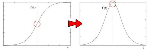
In the previous tutorial we learned how to use the Sobel Operator. It was based on the fact that in the edge area, the pixel intensity shows a “jump” or a high variation of intensity. Getting the first derivative of the intensity, we observed that an edge is characterized by a maximum, as it can be seen in the figure:
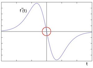
And...what happens if we take the second derivative?
You can observe that the second derivative is zero! So, we can also use this criterion to attempt to detect edges in an image. However, note that zeros will not only appear in edges (they can actually appear in other meaningless locations); this can be solved by applying filtering where needed.
Laplacian Operator
- From the explanation above, we deduce that the second derivative can be used todetect edges. Since images are “2D”, we would need to take the derivative in both dimensions. Here, the Laplacian operator comes handy.
- The Laplacian operator is defined by:
- The Laplacian operator is implemented in OpenCV by the function Laplacian. In fact, since the Laplacian uses the gradient of images, it calls internally the Sobeloperator to perform its computation.
Canny Edge Detector
Theory
- The Canny Edge detector was developed by John F. Canny in 1986. Also known to many as the optimal detector, Canny algorithm aims to satisfy three main criteria:
- Low error rate: Meaning a good detection of only existent edges.标识出尽可能多的实际边缘,同时尽可能的减少噪声产生的误报。
- Good localization: The distance between edge pixels detected and real edge pixels have to be minimized.标识出的边缘要与图像中的实际边缘尽可能接近。
- Minimal response: Only one detector response per edge.图像中的边缘只能标识一次。(最小响应)
- Find the gradient strength and direction with:计算梯度的幅值和方向
- The direction is rounded to one of four possible angles (namely 0, 45, 90 or 135)梯度方向近似到四个可能角度之一(一般 0, 45, 90, 135)
suppression
生词本去背诵英 [səˈpreʃn]美 [səˈprɛʃən]analogous
生词本英 [əˈnæləgəs]美 [əˈnæləɡəs]gradient strength
Non-maximum suppression is applied. This removes pixels that are not considered to be part of an edge. Hence, only thin lines (candidate edges) will remain.
Hysteresis: The final step. Canny does use two thresholds (upper and lower):
- If a pixel gradient is higher than the upper threshold, the pixel is accepted as an edge
- If a pixel gradient value is below the lower threshold, then it is rejected.
- If the pixel gradient is between the two thresholds, then it will be accepted only if it is connected to a pixel that is above the upper threshold.
Canny recommended a upper:lower ratio between 2:1 and 3:1.
For more details, you can always consult your favorite Computer Vision book.
非极大值 抑制。 这一步排除非边缘像素, 仅仅保留了一些细线条(候选边缘)。
滞后阈值: 最后一步,Canny 使用了滞后阈值,滞后阈值需要两个阈值(高阈值和低阈值):
- 如果某一像素位置的幅值超过 高 阈值, 该像素被保留为边缘像素。
- 如果某一像素位置的幅值小于 低 阈值, 该像素被排除。
- 如果某一像素位置的幅值在两个阈值之间,该像素仅仅在连接到一个高于 高 阈值的像素时被保留。
Canny 推荐的 高:低 阈值比在 2:1 到3:1之间。
想要了解更多细节,你可以参考任何你喜欢的计算机视觉书籍。

Cartesian
生词本polar
生词本Hough Line Transform
Goal
In this tutorial you will learn how to:
- Use the OpenCV functions HoughLines and HoughLinesP to detect lines in an image.使用opencv函数HoughLines和HoughLinesP检测图像中的直线。
Theory
Note
The explanation below belongs to the book Learning OpenCV by Bradski and Kaehler.
Hough Line Transform
- The Hough Line Transform is a transform used to detect straight lines.霍夫线性变换是一个用于检测直线的变换。
- To apply the Transform, first an edge detection pre-processing is desirable.进行霍夫变换前,首先要进行边缘检测。
How does it work?
As you know, a line in the image space can be expressed with twovariables.For example:众所周知,图像空间中的直线能够用两个变量表达。
- In the Cartesian coordinate system: Parameters:
 .笛卡尔坐标系(斜率和截距)
 - In the Polar coordinate system: Parameters:
 极坐标系统(极径和极角)
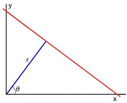
For Hough Transforms, we will express lines in the Polar system. Hence, a line equation can be written as:
在霍夫变换中,我们用极坐标来表示直线,直线方程如下表达:

- In the Cartesian coordinate system: Parameters:
Arranging the terms:整理
In general for each point
 , we can define the family of lines that goes through that point as:对于每一个点(x0,y0),我们定义一个线族,每一条线都穿过这个点。
一般来说对于点
 , 我们可以将通过这个点的一族直线统一定义为:(官方翻译)
Meaning that each pair
 represents each line that passes by .意思是,每一组点都代表一条线,这条线经过(x0,y0)。
这就意味着每一对
 代表一条通过点 的直线.(官方翻译)
sinusoid
英 ['saɪnəsɔɪd] 美 ['saɪnəˌsɔɪd]n.If for a given
we plot the family of lines that goes through it, we get a sinusoid. For instance, for  and
and  we get the following plot (in a plane
  -
-  ):
):如果对于一个给定点
我们在极坐标对极径极角平面绘出所有通过它的直线, 将得到一条正弦曲线. 例如, 对于给定点  and
and  我们可以绘出下图 (在平面
  -
-  ):(官方翻译)
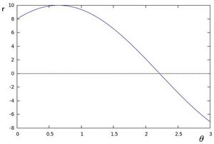
We consider only points such that
 and
and  .
.由于显卡的能力增强,现在的 OpenCV 已经有新的形态了,即大量的运算位于显卡上。
intersect
英 [ˌɪntə'sekt]美 [ˌɪntɚˈsɛkt]3.cWe can do the same operation above for all the points in an image. If the curves of two different pointsintersectin the plane
- , that means that both points belong to a same line. For instance, following with the example above and drawing the plot for two more points:  ,
,  and
and  ,
,  , we get:
我们为图像中所有的点重复以上的操作。如果两个不同点的弧度在平面
- 相交,这意味着,这两个点属于同一条线。例如,按照上面的例子画图,, and , , we get:我们可以对图像中所有的点进行上述操作.如果两个不同点进行上述操作后得到的曲线在平面
- 相交, 这就意味着它们通过同一条直线. 例如, 接上面的例子我们继续对点:  ,
,  和点
和点 ,
,  绘图, 得到下图: (官方翻译)
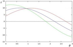
The three plots intersect in one single point
 , these coordinates are the parameters (
 ) or the line in which ,
  and
and  lay.
lay.这三条曲线在
- 平面相交于点(0.925,9.6),坐标表示参数对() 或者是说点 , 点  和点
和点  组成的平面内的的直线.
What does all the stuff above mean? It means that in general, a line can bedetected by finding the number of intersections between curves.The more curves intersecting means that the line represented by that intersection have more points. In general, we can define a threshold of the minimum number of intersections needed to detect a line.
那么以上的材料要说明什么呢? 这意味着一般来说, 一条直线能够通过在平面
- 寻找交于一点的曲线数量来 检测. 越多曲线交于一点也就意味着这个交点表示的直线由更多的点组成. 一般来说我们可以通过设置直线上点的 阈值 来定义多少条曲线交于一点我们才认为 检测 到了一条直线.This is what the Hough Line Transform does. It keepstrack of the intersection between curves of every point in the image. If the number of intersections is above some threshold, then it declares it as a line with the parameters
 of the intersection point.
这就是霍夫线变换要做的. 它追踪图像中每个点对应曲线间的交点. 如果交于一点的曲线的数量超过了 阈值, 那么可以认为这个交点所代表的参数对
 在原图像中为一条直线.
Standard and Probabilistic Hough Line Transform
OpenCV implements two kind of Hough Line Transforms:Opencv完成两种霍夫变换
- The Standard Hough Transform标准霍夫变换
- It consists in pretty much what we just explained in the previous section. It gives you as result a vector of couples
- In OpenCV it is implemented with the function HoughLines
- The Probabilistic Hough Line Transform 统计概率霍夫变换
- A more efficient implementation of the Hough Line Transform.It gives as output the extremes of the detected lines
它输出检测到的直线的端点
- In OpenCV it is implemented with the function HoughLinesP
For sake of efficiency, OpenCV implements a
Hough Circle Transform 还没明白
detection method slightly trickier than the standard Hough Transform:The Hough gradient method. For more details, please check the book Learning OpenCV or your favorite Computer Vision bibliography出于上面提到的对运算效率的考虑, OpenCV实现的是一个比标准霍夫圆变换更为灵活的检测方法: 霍夫梯度法, 也叫2-1霍夫变换(21HT), 它的原理依据是圆心一定是在圆上的每个点的模向量上, 这些圆上点模向量的交点就是圆心, 霍夫梯度法的第一步就是找到这些圆心, 这样三维的累加平面就又转化为二维累加平面. 第二部根据所有候选中心的边缘非0像素对其的支持程度来确定半径. 21HT方法最早在Illingworth的论文The Adaptive Hough Transform中提出并详细描述, 也可参照Yuen在1990年发表的A Comparative Study of Hough Transform Methods for Circle Finding, Bradski的《学习OpenCV》一书则对OpenCV中具体对算法的具体实现有详细描述并讨论了霍夫梯度法的局限性.Remapping重映射interpolation
生词本英 [ɪnˌtɜ:pə'leɪʃn]美 [ɪnˌtɚpəˈleʃən]Affine Transformations仿射变换
warpAffine
Applies an affine transformation to an image.
- C++: void warpAffine(InputArray src, OutputArray dst, InputArray M, Sizedsize, int flags=INTER_LINEAR, int borderMode=BORDER_CONSTANT, const Scalar&borderValue=Scalar())
- Python: cv2.warpAffine(src, M, dsize[, dst[, flags[, borderMode[, borderValue]]]]) → dst
- C: void cvWarpAffine(const CvArr* src, CvArr* dst, const CvMat* map_matrix, int flags=CV_INTER_LINEAR+CV_WARP_FILL_OUTLIERS, CvScalar fillval=cvScalarAll(0))
- Python: cv.WarpAffine(src, dst, mapMatrix, flags=CV_INTER_LINEAR+CV_WARP_FILL_OUTLIERS, fillval=(0, 0, 0, 0)) → None
- C: void cvGetQuadrangleSubPix(const CvArr* src, CvArr* dst, const CvMat*map_matrix)
- Python: cv.GetQuadrangleSubPix(src, dst, mapMatrix) → None
Parameters:
- src – input image.
- dst – output image that has the size dsize and the same type as src .
- M –
transformation matrix.
- dsize – size of the output image.
- flags – combination of interpolation methods (see resize()) and the optional flag WARP_INVERSE_MAP that means that M is the inverse transformation (
).
- borderMode – pixel extrapolation method (seeborderInterpolate()); when borderMode=BORDER_TRANSPARENT , it means that the pixels in the destination image corresponding to the “outliers” in the source image are not modified by the function.
- borderValue – value used in case of a constant border; by default, it is 0.
The function warpAffine transforms the source image using the specified matrix:
when the flag WARP_INVERSE_MAP is set. Otherwise, the transformation is first inverted with invertAffineTransform() and then put in the formula above instead of M . The function cannot operate in-place.
See also
warpPerspective(), resize(), remap(), getRectSubPix(),transform()
Note
cvGetQuadrangleSubPix is similar to cvWarpAffine, but the outliers are extrapolated using replication border mode.
isotropic
生词本英 [ˌaɪsə'trɒpɪk]美 [ˌaɪsə'trɒpɪk]getRotationMatrix2D
Calculates an affine matrix of 2D rotation.
- C++: Mat getRotationMatrix2D(Point2f center, double angle, double scale)
- Python: cv2.getRotationMatrix2D(center, angle, scale) → retval
- C: CvMat* cv2DRotationMatrix(CvPoint2D32f center, double angle, doublescale, CvMat* map_matrix)
- Python: cv.GetRotationMatrix2D(center, angle, scale, mapMatrix) → None
Parameters:
- center – Center of the rotation in the source image.
- angle – Rotation angle in degrees. Positive values mean counter-clockwise rotation (the coordinate origin is assumed to be the top-left corner).
- scale – Isotropic scale factor.
- map_matrix – The output affine transformation, 2x3 floating-point matrix.
The function calculates the following matrix:
where
The transformation maps the rotation center to itself. If this is not the target, adjust the shift.
equalize 英 ['i:kwəlaɪz] 美 [ˈikwəˌlaɪz]
vt.& vi.representation 英 [ˌreprɪzenˈteɪʃn] 美 [ˌrɛprɪzɛnˈteʃən]
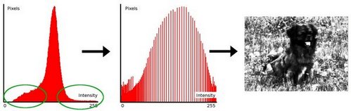
n.Take a look at the figure below: The green circles indicate the underpopulated intensities.quantify 英 ['kwɒntɪfaɪ]美 ['kwɑ:ntɪfaɪ]
vt.spread 英 [spred] 美 [sprɛd]
accomplish 英 [ə'kʌmplɪʃ] 美 [əˈkɑmplɪʃ]
cumulative 英 ['kju:mjələtɪv] 美 [ˈkjumjəˌletɪv, -jələtɪv]
adj.remapping英 [rɪ'mæpɪŋ] 美 [rɪ'mæpɪŋ]
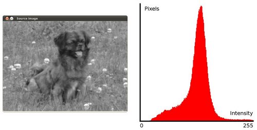
重测图What is an Image Histogram?
- It is agraphical representationof theintensity distributionof an image.图像中强度分布的图形表达式
- It quantifies the number of pixels for each intensity value considered.
- 它(直方图)统计每种强度值的像素个数。
What is Histogram Equalization?直方图均衡
- It is a method that improves the contrast in an image,in order tostretch out the intensity range.
- 它是一种方法,通过拉伸(图像)强度分布,提升图像的对比度,
- To make it clearer, from the image above, you can see that the pixels seem clustered around the middle of
- the available range of intensities. What Histogram Equalization does is to stretch out this range. Take a
- look at the figure below: The green circles indicate the underpopulated intensities. After applying the
- equalization, we get an histogram like the figure in the center. The resulting image is shown in the
- picture at right.
- 从上面的图像,我们看到,像素值都聚集强度分布的中间区域。直方图均衡就是拉伸这个中间区域。我们看下图:绿色
- 圆圈表示低强度分布区域。通过均衡,我们得到中间所示的直方图。结果图像显示在其右侧。
How does it work?
blur()
Equalization implies mapping one distribution (the given histogram) to another distribution
(a wider and more uniform distribution of intensity values) so the intensity values are spreaded
over the whole range.
均衡将分布从一个映射到另一个,所以强灰度值被分布到整个区域。
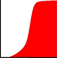
To accomplish the equalization effect, the remapping should be the cumulative distribution function
(cdf) (more details, refer to Learning OpenCV). For the histogram
, its cumulative distribution
is:
为了完成均衡,映射是建增的分布函数。直方图H(i),它的整体分布是:
要使用其作为映射函数, 我们必须对最大值为255 (或者用图像的最大强度值) 的累积分布
进行归一化.
同上例, 累积分布函数为:
To use this as a remapping function, we have to normalize
( or the maximum value for the intensity of the image ). From the example above, the cumulative
function is:
使用这个作为重映射函数,我们将最大值进行均匀分布,从上面的例子来看,
Finally, we use a simple remapping procedure to obtain the intensity values of the equalized image:
最后,我们使用一个简便的重映射过程去获得均衡化图像的直方图。
Histogram Calculation直方图计算
Goal
correspondent
生词本去背诵英 [ˌkɒrəˈspɒndənt]美 [ˌkɔrɪˈspɑndənt, ˌkɑr-]In this tutorial you will learn how to:
- Use the OpenCV function split to divide an image into its correspondent planes.
- 使用函数split将图像分成相应的平面。分割成单通道数组
- To calculate histograms of arrays of images by using the OpenCV function calcHist。
- 使用calcHist函数统计每组图像的直方图。计算图像阵列的直方图
- To normalize an array by using the function normalize
- 使用函数normalize均匀化数组。归一化数组
Note
In the last tutorial (Histogram Equalization) we talked about a particular kind of histogram called
Image histogram. Now we will considerate it in itsmore general concept. Read on!
在上一篇中(直方图均衡化)我们介绍了一种特殊直方图叫做图像直方图。现在我们从更加广义的角度来考虑直方图的概念,继续往下读。
What are histograms?
Histograms are collected counts of data organized into a set of predefined bins
直方图就是将统计好的数据存入bins数组,直方图是对数据的集合统计,并将统计结果分布于一系列预定义的bins中。
When we say data we are not restricting it to be intensity values (as we saw in the previous Tutorial).
The data collected can be whatever feature you find useful to describe your image.
当我们谈到数据,我们没有严格的说是灰度值,
统计数据可能是任何能有效描述图像的特征。
Let’s see an example. Imagine that a Matrix contains information of an image (i.e. intensity in the
range
):
先看一个例子吧。 假设有一个矩阵包含一张图像的信息 (灰度值
):
What happens if we want to count this datain an organized way? Since we know that the range of information
value for this case is 256 values, we can segment our range in subparts (called bins) like:
如果我们按照某种方式去统计这些数字,会发生什么情况呢?既然已知数字的范围包含256个值,我们可以将这个范围分割
成子区域。
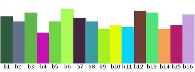
and we can keep count of the number of pixels that fall in the range of each
. Applying this to the
example above we get the image below ( axis x represents the bins and axis y the number of pixels in each
of them).
我们可以将像素的统计数放入相应的bin区域。将其应用到下面的例子中。(x轴表示bins,y轴表示相应bins区域的像素数)
This was just a simple example of how an histogram works and why it is useful. An histogram can keep count
not only of color intensities, but of whatever image features that we want to measure (i.e. gradients,
directions, etc).
这仅仅是用来说明直方图如何工作的一个实例。一个直方图不仅可以统计色彩强度,而且可以统计任何我们想要度量的图像特
性(比如:梯度,方向等等)。
Let’s identify some parts of the histogram:让我们来搞清楚直方图的一些具体细节:
- dims: The number of parameters you want to collect data of. In our example, dims = 1 because we are only
- counting the intensity values of each pixel (in a greyscale image).
- 我们想要统计的特征的数目。(在上例中,dims = 1因为我们仅仅统计了灰度值(灰度级图像)
- bins: It is the number of subdivisions in each dim. In our example, bins = 16
- 每一维的分区数,我们的示例是16(每个特征空间子区段的数目)
- range: The limits for the values to be measured. In this case: range = [0,255]
- 我们所度量的值的范围,本例是【0-255】(每个特征空间的取值范围)
What if you want to count two features? In this case your resulting histogram would be a 3D plot (in which x
and y would be
and
for each feature and z would be the number of counts for each combination of
. The same would apply for more features (of course it gets trickier)
怎样去统计两个特征呢?在这种情况下,直方图就是3维的了,x轴和y轴分别代表一个特征,z轴是调入(binx, biny)组合
的样本数。同样的方法适用于更高维的情形(当然会变得很复杂)。
segment
生词本去背诵英 [ˈsegmənt]美 [ˈsɛɡmənt]what if
生词本英 [hwɔt if]美 [hwɑt ɪf]What OpenCV offers you
For simple purposes, OpenCV implements the function calcHist, which calculates the histogram of a set of
arrays (usually images or image planes). It can operate with up to 32 dimensions. We will see it in the
code below!
opencv提供了一个简单的计算数组集(通常是图像或分割后的通道)的直方图函数calcHist。支持高达32维的直方图。下面的代码演示了
如何使用该函数计算直方图。
Code
What does this program do?
- Loads an image
- Splits the image into its R, G and B planes using the function split
- Calculate the Histogram of each 1-channel plane by calling the function calcHist计算各单通道图像的直方图
- Plot the three histograms in a window在一个窗口叠加显示3张直方图
Histogram Comparison
In this tutorial you will learn how to:
- Use the function compareHist toget a numerical parameter that express how well two histograms match with each other.
- 使用函数获得一个数字参数来表示两个直方图的对比(相似度)。
- Use different metrics to compare histograms
- 使用不同的方法(对比标准)去度量这两个直方图。
Theory
To compare two histograms (
and
), first we have to choose a metric (
) to expresshow well
both histograms match.
对比这两个直方图,首先我们要选择一个衡量直方图相似度的对比标准()
OpenCV implements the function compareHist to perform a comparison. It also offers 4 different metrics to
compute the matching:
opencv 使用函数compareHist来完成对比。opencv 还提供了4中不同的对比标准去计算相似度。
Correlation ( CV_COMP_CORREL )
where
and
is the total number of histogram bins.
Chi-Square ( CV_COMP_CHISQR )
Intersection ( method=CV_COMP_INTERSECT )
Bhattacharyya distance ( CV_COMP_BHATTACHARYYA )
It is reported that a bus went out of control on a highwaysouth of the city last night.名(south前有介词或定冠词)、副词(south前有无)Code
What does this program do?
- Loads a base image and 2 test images to be compared with it.
- Generate 1 image that is the lower half of the base image
- Convert the images to HSV format
- Calculate the H-S histogram for all the images and normalize them in order to compare them.
- Compare the histogram of the base image with respect to the 2 test histograms, the histogram of the lower half base image and with the same base image histogram.
- Display the numerical matching parameters obtained.
- at sight 第一眼
- To tell truth 讲实话
- at a loss 不知所措
- out of control失去控制
word = news消息,不可数,the driver was at a loss when word came that he was forbidden to drive for speeding.There is a Liu chang(表达人不清晰,a表示某一个概念,相当于some=a certain) in our class , but i am afraid he isn't the one you want.As is known to all, the (普通名词+专有名词=专有名词)People's(普通名词) Republic of China (专有名词)is the biggest(最高级) developing country in the world.We are now living in the(特指) "information(普通名词) age(普通名词)"(普通名词+普通名词=表示一个时代),a time(所有时代之一) of new discoveries(复数) and great changes.make time抽出时间 make time in her day for regular sport.On February 27, 2011, Premier Wen Jiabao hold an online chat with Internet users across the country(特指中国) and overseas.the third time the leader had participated in the event.we work together to achieve our common purpose :a world that is safer ,cleaner more thanthe one we found.China held a ceremory to commemorate anniversary of xinhai Revolution at the (普通名词+专有名词)Great Hall of the People in Beijing.As (\)cities (名复数表泛指)grow, so does the number of buildings that characterize them: office factories . shopping centers and high-rise apartment buildings.in danger of ...处于危险之中People who drink and drive are a danger both to themselves and to others. They are in danger of losing their lives.According to recent reports the rare animals, the crocodile, will be in


![\begin{array}{l}[0, 255] = { [0, 15] \cup [16, 31] \cup ....\cup [240,255] } \\range = { bin_{1} \cup bin_{2} \cup ....\cup bin_{n = 15} }\end{array}](http://docs.opencv.org/2.4/_images/math/c73157b35da93244fa5489fc51b92217c199bea7.png)


- open cv+C++错误及经验总结(七)
- open cv+C++错误及经验总结(四)
- open cv+C++错误及经验总结(五)
- open cv+C++错误及经验总结(六)
- open cv+C++错误及经验总结(八)
- open cv+C++错误及经验总结(九)
- open cv+C++错误及经验总结(十)
- open cv+C++错误及经验总结(十一)
- open cv+C++错误及经验总结(十二)
- open cv+C++错误及经验总结(十三)
- open cv+C++错误及经验总结(十四)
- open cv+C++错误及经验总结(二)
- open cv+C++错误及经验总结(三)
- Open CV 学习经验总结
- open cv+C++错误总结(一)
- Open CV
- open cv
- Open CV学习记录(七)——图片B、G、R成分的分离与合并
- jQuery动态创建div方法
- html5移动开发物理游戏的心得
- jstl标签: c:Foreach详解
- 关于html中table容易出现的问题
- 分治法,棋盘覆盖
- open cv+C++错误及经验总结(七)
- 恢复Chrome打开新的标签页的方法
- [Android问答] px、dp和sp,这些单位有什么区别?
- LeetCode 053 Maximum Subarray
- Java类型检查
- 图像特征检测
- java.net.SocketException: sendto failed: EPIPE (Broken pipe)
- python学习笔记之(五)
- html5移动开发物理游戏的方法心得