Whitening&PCA
来源:互联网 发布:三菱触摸屏怎么存数据 编辑:程序博客网 时间:2024/05/16 08:19
Whitening
Contents
[hide]- 1Introduction
- 22D example
- 3ZCA Whitening
- 4Regularizaton
Introduction
We have used PCA to reduce the dimension of the data. There is a closely related preprocessing step calledwhitening (or, in some other literatures,sphering)which is needed for some algorithms. If we are training on images,the raw input isredundant,since adjacent pixel valuesare highly correlated. The goal of whitening is to make the input less redundant; more formally,our desiderata are that our learning algorithms sees a training input where (i) the features areless correlated with each other, and (ii) the features all have thesame variance.
2D example
We will first describe whitening using our previous 2D example. We will then describe how this can be combined with smoothing, and finally how to combinethis with PCA.
How can we make our input features uncorrelated with each other? We had already done this when computing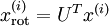 . Repeating our previous figure, our plot for
 was:
was:
The covariance matrix of this data is given by:
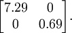
(Note: Technically, many of thestatements in this section about the "covariance" will be true only if the datahas zero mean. In the rest of this section, we will take this assumption asimplicit in our statements. However, even if the data's mean isn't exactly zero, the intuitions we're presenting here still hold true, and so this isn't somethingthat you should worry about.)
It is no accident that the diagonal values are and
and . Further, the off-diagonal entries are zero; thus,
 and
and are uncorrelated, satisfying one of our desiderata for whitened data (that the features be less correlated).
To make each of our input features have unit variance, we can simply rescaleeach feature by
by . Concretely, we defineour whitened data
 as follows:
Plotting , we get:
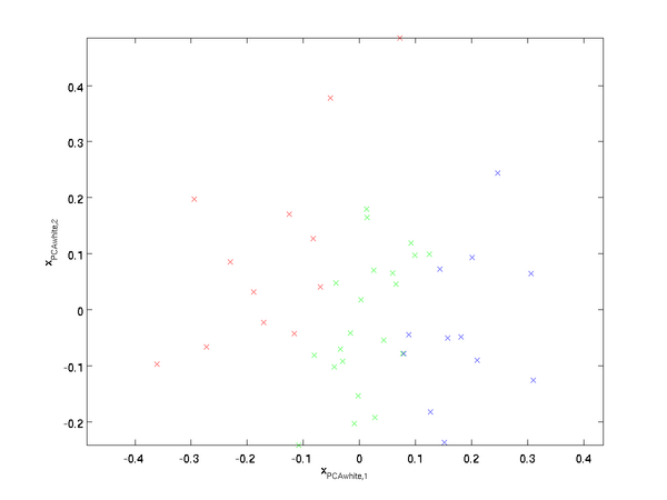
This data now has covariance equal to the identity matrix . We say that is ourPCA whitened version of the data: The different components of are uncorrelated and have unit variance.
Whitening combined with dimensionality reduction. If you want to have data that is whitened and which is lower dimensional thanthe original input, you can also optionally keep only the top  components of.When we combine PCA whitening with regularization(described later), the last few components of will be nearly zero anyway, and thus can safely be dropped.
ZCA Whitening
Finally, it turns out that this way of getting the data to have covariance identityisn't unique. Concretely, if  is any orthogonal matrix, so that it satisfies
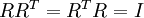 (less formally,if is a rotation/reflection matrix),then
 will also have identity covariance. InZCA whitening,we choose
 .We define

Plotting , we get:
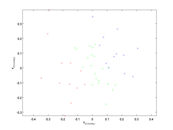
It can be shown that out of all possible choices for, this choice of rotation causes to be as close as possible to the original input data .
.
When using ZCA whitening (unlike PCA whitening), we usually keep all dimensionsof the data, and do not try to reduce its dimension.
Regularizaton
When implementing PCA whitening or ZCA whitening in practice, sometimes some of the eigenvalues will be numerically close to 0, and thus the scaling step where we divide by
 would involve dividing by a value close to zero; this may cause the data to blow up (take on large values) or otherwise be numerically unstable.In practice, we therefore implement this scaling step using a small amount of regularization, andadd a small constant
 to the eigenvalues before taking their square root and inverse:
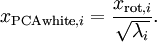
When takes values around![\textstyle [-1,1]](http://ufldl.stanford.edu/wiki/images/math/8/5/a/85a1c5a07f21a9eebbfb1dca380f8d38.png) , a value of
, a value of might be typical.
For the case of images, adding here alsohas the effect of slightly smoothing (or low-pass filtering) the input image. Thisalso has a desirable effect of removing aliasing artifacts caused by the way pixels are laid out in an image, and can improve the features learned (details are beyond the scope of these notes).
ZCA whitening is a form of pre-processing of the data that maps it from to. It turns out that this is also a rough model of how the biological eye (the retina) processes images. Specifically, as your eye perceives images, most adjacent "pixels" in your eye will perceive very similar values, since adjacent parts of an image tend to be highly correlatedin intensity. It is thus wasteful for your eye to have to transmit every pixel separately (via your optic nerve) to your brain. Instead, your retina performs a decorrelation operation (this is done via retinal neurons that compute a function called "on center, off surround/off center, on surround") which is similar to that performed by ZCA. This results in a less redundant representation of the input image, which is then transmitted to your brain.
PCA
Contents
[hide]- 1Introduction
- 2Example and Mathematical Background
- 3Rotating the Data
- 4Reducing the Data Dimension
- 5Recovering an Approximation of the Data
- 6Number of components to retain
- 7PCA on Images
- 8References
Introduction
Principal Components Analysis (PCA) is a dimensionality reduction algorithm that can be used to significantlyspeed up your unsupervised feature learning algorithm. More importantly, understanding PCA will enable us to later implementwhitening, which is an important pre-processing step for manyalgorithms.
Suppose you are training your algorithm on images. Then the input will be somewhat redundant, because the values of adjacent pixels in an image are highly correlated. Concretely, suppose we are training on 16x16 gray scaleimage patches. Then are 256 dimensional vectors, with one feature
 corresponding to the intensity of each pixel. Because of the correlation between adjacent pixels, PCA will allow us to approximate the input with a much lower dimensional one, while incurring very little error.
Example and Mathematical Background
For our running example, we will use a dataset  with
with dimensional inputs, so that
 .Suppose we want to reduce the data from 2 dimensions to 1. (In practice, we might want to reduce data from 256 to 50 dimensions, say; but using lower dimensional data in our example allows us to visualize the algorithms better.) Here is our dataset:
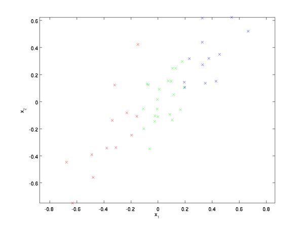
This data has already been pre-processed so that each of the features  and
and have about the same mean (zero) and variance.
For the purpose of illustration, we have also colored each of the points one of three colors, depending on their value; these colors are not used by the algorithm, and are for illustration only.
PCA will find a lower-dimensional subspace onto which to project our data. From visually examining the data, it appears that is the principal direction of variation of the data, and
 the secondary direction of variation:
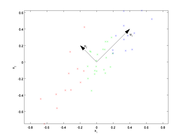
I.e., the data varies much more in the direction than. To more formally find the directions and, we first compute the matrix as follows:
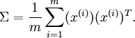
If has zero mean, then is exactly the covariance matrix of. (The symbol "", pronounced "Sigma", is the standard notation for denoting the covariance matrix. Unfortunately it looks just like the summation symbol, as in ; but these are two different things.)
It can then be shown that ---the principal direction of variation of the data---is the top (principal) eigenvector of , and is the second eigenvector.
Note: If you are interested in seeing a more formal mathematical derivation/justification of this result, see the CS229 (Machine Learning) lecture notes on PCA (link at bottom of this page). You won't need to do so to follow along this course, however.
You can use standard numerical linear algebra software to find these eigenvectors (see Implementation Notes).Concretely, let us compute the eigenvectors of, and stack the eigenvectors in columns to form the matrix :
:
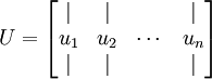
Here, is the principal eigenvector (corresponding to the largest eigenvalue), is the second eigenvector, and so on. Also, let 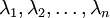 be the corresponding eigenvalues.
The vectors and in our example form a new basis in which we can represent the data. Concretely, let be some training example. Then
 is the length (magnitude) of the projection of onto the vector.
Similarly,  is the magnitude of projected onto the vector.
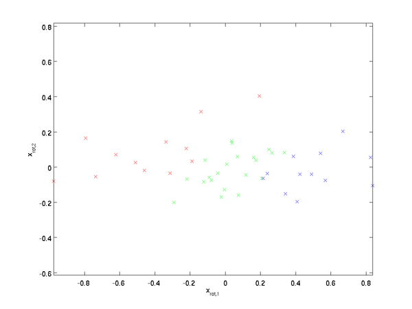
Rotatingthe Data
Thus, we can represent in the -basis by computing
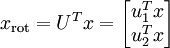
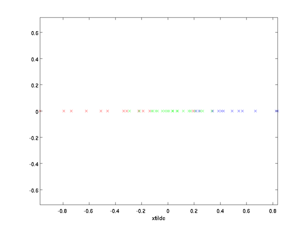
(The subscript "rot" comes from the observation that this corresponds to a rotation (and possibly reflection) of the original data.)Lets take the entire training set, and compute for every . Plotting this transformed data, we get:
This is the training set rotated into the , basis. In the general case,  will be the training set rotated into the basis,, ...,
 .
.
One of the properties of is that it is an "orthogonal" matrix, which means that it satisfies  . So if you ever need to go from the rotated vectors back to the original data, you can compute

because  .
.
Reducing the Data Dimension
We see that the principal direction of variation of the data is the first dimension of this rotated data. Thus, if we want to reduce this data to one dimension, we can set
More generally, if  and we want to reduce it to a dimensional representation
 (where
 ), we would take the first components of, which correspond to the top directions of variation.
Another way of explaining PCA is that is an dimensional vector, where the first few components are likely to be large (e.g., in our example, we saw that takes reasonably large values for most examples), and the later components are likely to be small (e.g., in our example,
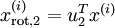 was more likely to be small). What PCA does it it drops the the later (smaller) components of, and just approximates them with 0's. Concretely, our definition of
 can also be arrived at by using anapproximation to
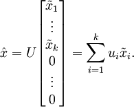
  where all but the first components are zeros.In other words, we have:
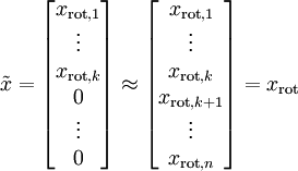
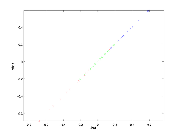
In our example, this gives us the following plot of (using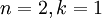 ):
):
However, since the final  components of as defined above would always be zero, there is no need to keep these zeros around, and so we define as a-dimensional vector with just the first (non-zero) components.
This also explains why we wanted to express our data in the basis:Decidingwhich components to keep becomes just keeping the top components. When we do this, we also say that we are "retaining the top PCA (or principal) components."
Recovering an Approximation of the Data
Now, is a lower-dimensional, "compressed" representationof the original. Given, how can we recover an approximation to the original value of? From anearlier section, we know that
  . Further, we can think of as an approximation to, where we have set the last components to zeros. Thus, given, we can pad it out with zeros to get our approximation to
 . Finally, we pre-multiplyby to get our approximation to. Concretely, we get
The final equality above comes from the definition of given earlier.(In a practical implementation, we wouldn't actually zero pad and then multiplyby, since that would mean multiplying a lot of things by zeros; instead,we'd just multiply with the first columns of as in the final expression above.)Applying this to our dataset, we get the following plot for:
We are thus using a 1 dimensional approximation to the original dataset.
If you are training an autoencoder or other unsupervised feature learning algorithm,the running time of your algorithm willdepend on the dimension of the input.If you feedinto your learning algorithm instead of, then you'll be training on a lower-dimensional input, and thus your algorithm might run significantly faster.For many datasets,the lower dimensional representation can be an extremely good approximation to the original, and using PCA this way can significantly speed up your algorithm while introducing very little approximation error.
Number of components to retain
How do we set ; i.e., how many PCA components should we retain? In our simple 2 dimensional example, it seemed natural to retain 1 out of the 2components, but for higher dimensional data, this decision isless trivial. If istoo large, then we won't be compressing the data much; in the limit of ,then we're just using the original data (but rotated into a different basis).Conversely, if istoo small, then we might be using a very bad approximation to the data.
To decide how to set , we will usually look at thepercentage of variance retained for different values of .Concretely, if, then we have an exact approximation to the data, and we say that 100% of the variance is retained. I.e., all of the variation of the original data is retained. Conversely, if , then we are approximating all the data with the zero vector,and thus 0% of the variance is retained.
More generally, let be the eigenvalues of (sorted in decreasing order), so that is the eigenvalue corresponding to the eigenvector
 . Then if we retain principal components, the percentage of variance retained is given by:

In our simple 2D example above,  , and
, and . Thus,by keeping only
 principal components, we retained
 ,or 91.3% of the variance.
A more formal definition of percentage of variance retainedis beyond the scope of these notes. However, it is possible to show that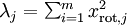 . Thus, if
 , that shows that
 is usually near 0 anyway, and we lose relatively little by approximating it with a constant 0. This also explains why we retain the top principal components (corresponding to the larger values of) instead of the bottomones. The top principal components are the ones that're more variable and that take on larger values, and for which we would incur a greater approximation error if we were to set them to zero.
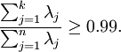
In the case of images, one common heuristic is to choose so as to retain 99% of the variance. In other words, we pick the smallest value of that satisfies
Depending on the application, if you are willing to incur some additional error, values in the 90-98% range are also sometimes used. When you describe to others how you applied PCA, saying that you chose to retain 95% of the variance will also be a much more easily interpretable description than saying that you retained 120 (or whatever other number of) components.
PCA on Images
For PCA to work, usually we want each of the features 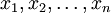 to have a similar range of values to the others (and to have a mean close to zero). If you've used PCA on other applications before, you may therefore have separatelypre-processed each feature to have zero mean and unit variance, by separately estimating the mean and variance of each feature.However,this isn't the pre-processing that we will apply to most types of images. Specifically,suppose we are training our algorithm onnatural images, so that is the value of pixel
 . By "natural images," we informally mean the type of image that a typical animal or person might see over their lifetime.
Note: Usually we use images of outdoor scenes with grass, trees, etc., and cut out small (say 16x16) image patches randomly from these to train the algorithm. But in practice most feature learning algorithms are extremely robust to the exact type of image it is trained on, so most images taken with a normal camera, so long as they aren't excessively blurry or have strange artifacts, should work.
When training on natural images, it makes little sense to estimate a separate mean and variance for each pixel, because the statistics in one part of the image should (theoretically) be the same as any other. This property of images is calledstationarity.
In detail, in order for PCA to work well, informally we require that (i) The features have approximatelyzero mean, and (ii) The different features havesimilar variances to each other. With natural images, (ii) is already satisfied even without variance normalization, and so we won't perform any variance normalization. (If you are training on audio data---say, on spectrograms---or on text data---say, bag-of-word vectors---we will usually not perform variance normalization either.) In fact, PCA is invariant to the scaling of the data, and will return the same eigenvectors regardless of the scaling of the input. More formally, if you multiply each feature vector by some positive number (thus scaling every feature in every training example by the same number), PCA's output eigenvectors will not change.
So, we won't use variance normalization. The only normalization we need to perform then ismean normalization, to ensure that the featureshave a mean around zero. Depending on the application, very often we are not interested in how bright the overall input image is. For example, in object recognition tasks, the overall brightness of the image doesn't affect what objectsthere are in the image. More formally, we are not interested in the mean intensity value of an image patch; thus, we can subtract out this value,as a form of mean normalization.
Concretely, if  are the (grayscale) intensity values of a 16x16 image patch (
 ), we might normalize the intensity of each image
 as follows:
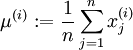
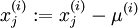 , for all
Note that the two steps above are done separately for each image ,and that here is the mean intensity of the image. In particular,this is not the same thing as estimating a mean value separately for each pixel.
If you are training your algorithm on images other than natural images (for example, images of handwritten characters, or images of single isolated objects centered against a white background),other types of normalization might be worth considering, and the best choice may be application dependent. But when training on natural images, using the per-image mean normalization method as given in the equations above would be a reasonable default.
References
http://cs229.stanford.edu
Implementing PCA/Whitening
In this section, we summarize the PCA, PCA whitening and ZCA whitening algorithms,and also describe how you can implement them using efficient linear algebra libraries.
First, we need to ensure that the data has (approximately) zero-mean. For natural images, we achieve this (approximately) by subtracting the mean value of each image patch.
We achieve this by computing the mean for each patch and subtracting it for each patch. In Matlab, we can do this by using
avg = mean(x, 1); % Compute the mean pixel intensity value separately for each patch. x = x - repmat(avg, size(x, 1), 1);
Next, we need to compute  . If you're implementing this in Matlab (or even if you're implementing this in C++, Java, etc., but have access to an efficient linear algebra library), doing it as an explicit sum is inefficient. Instead, we can compute this in one fell swoop as
sigma = x * x' / size(x, 2);
(Check the math yourself for correctness.) Here, we assume that x is a data structure that contains one training example per column (so,x is a-by- matrix).
Next, PCA computes the eigenvectors of Σ. One could do this using the Matlabeig function. However, becauseΣ is a symmetric positive semi-definite matrix, it is more numerically reliable to do this using thesvd function. Concretely, if you implement
[U,S,V] = svd(sigma);
then the matrix U will contain the eigenvectors ofSigma (one eigenvector per column, sorted in order from top to bottom eigenvector), and the diagonal entries of the matrixS will contain the corresponding eigenvalues (also sorted in decreasing order). The matrixV will be equal to transpose ofU, and can be safely ignored.
(Note: The svd function actually computes the singular vectors and singular values of a matrix, which for the special case of a symmetric positive semi-definite matrix---which is all that we're concerned with here---is equal to its eigenvectors and eigenvalues. A full discussion of singular vectors vs. eigenvectors is beyond the scope of these notes.)
Finally, you can compute and as follows:
xRot = U' * x; % rotated version of the data. xTilde = U(:,1:k)' * x; % reduced dimension representation of the data, % where k is the number of eigenvectors to keep
This gives your PCA representation of the data in terms of . Incidentally, ifx is a -by- matrix containing all your training data, this is a vectorizedimplementation, and the expressionsabove work too for computingxrot and for your entire training setall in one go. The resultingxrot and will have one column corresponding to each training example.
To compute the PCA whitened data  , use
, use
xPCAwhite = diag(1./sqrt(diag(S) + epsilon)) * U' * x;
Since S's diagonal contains the eigenvalues, this turns out to be a compact way of computing simultaneously for all.
Finally, you can also compute the ZCA whitened data as:
xZCAwhite = U * diag(1./sqrt(diag(S) + epsilon)) * U' * x;
Implementing PCA/Whitening
In this section, we summarize the PCA, PCA whitening and ZCA whitening algorithms,and also describe how you can implement them using efficient linear algebra libraries.
First, we need to ensure that the data has (approximately) zero-mean. For natural images, we achieve this (approximately) by subtracting the mean value of each image patch.
We achieve this by computing the mean for each patch and subtracting it for each patch. In Matlab, we can do this by using
avg = mean(x, 1); % Compute the mean pixel intensity value separately for each patch. x = x - repmat(avg, size(x, 1), 1);
Next, we need to compute . If you're implementing this in Matlab (or even if you're implementing this in C++, Java, etc., but have access to an efficient linear algebra library), doing it as an explicit sum is inefficient. Instead, we can compute this in one fell swoop as
sigma = x * x' / size(x, 2);
(Check the math yourself for correctness.) Here, we assume thatx is a data structure that contains one training example per column (so,x is a-by- matrix).
Next, PCA computes the eigenvectors of Σ. One could do this using the Matlabeig function. However, becauseΣ is asymmetric positive semi-definite matrix, it is more numerically reliable to do this using thesvd function. Concretely, if you implement
[U,S,V] = svd(sigma);
then the matrix U will contain the eigenvectors ofSigma (one eigenvector per column, sorted in order from top to bottom eigenvector), and the diagonal entries of the matrixS will contain the corresponding eigenvalues (also sorted in decreasing order). The matrixV will be equal to transpose ofU, and can be safely ignored.
(Note: The svd function actually computes the singular vectors and singular values of a matrix, which for the special case of a symmetric positive semi-definite matrix---which is all that we're concerned with here---is equal to its eigenvectors and eigenvalues. A full discussion of singular vectors vs. eigenvectors is beyond the scope of these notes.)
Finally, you can compute and as follows:
xRot = U' * x; % rotated version of the data. xTilde = U(:,1:k)' * x; % reduced dimension representation of the data, % where k is the number of eigenvectors to keep
This gives your PCA representation of the data in terms of . Incidentally, ifx is a -by- matrix containing all your training data, this is a vectorizedimplementation, and the expressionsabove work too for computingxrot and for your entire training setall in one go. The resultingxrot and will have one column corresponding to each training example.
To compute the PCA whitened data , use
xPCAwhite = diag(1./sqrt(diag(S) + epsilon)) * U' * x;
Since S's diagonal contains the eigenvalues, this turns out to be a compact way of computingsimultaneously for all.
Finally, you can also compute the ZCA whitened data as:
xZCAwhite = U * diag(1./sqrt(diag(S) + epsilon)) * U' * x;
PCA and Whitening on natural images
In this exercise, you will implement PCA, PCA whitening and ZCA whitening, and apply them to image patches taken from natural images.
You will build on the MATLAB starter code which we have provided in pca_exercise.zip. You need only write code at the places indicated by "YOUR CODE HERE" in the files. The only file you need to modify ispca_gen.m.
Step 0: Prepare data
Step 0a: Load data
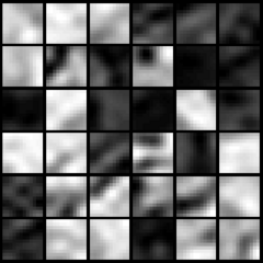
The starter code contains code to load a set of natural images and sample 12x12 patches from them. The raw patches will look something like this:

These patches are stored as column vectors  in the
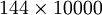 matrixx.
Step 0b: Zero mean the data
First, for each image patch, compute the mean pixel value and subtract it from that image, this centering the image around zero. You should compute a different mean value for each image patch.
Step 1: Implement PCA
Step 1a: Implement PCA
In this step, you will implement PCA to obtain xrot, the matrix in which the data is "rotated" to the basis comprising the principal components (i.e. the eigenvectors ofΣ). Note that in this part of the exercise, you shouldnot whiten the data.
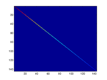
Step 1b: Check covariance
To verify that your implementation of PCA is correct, you should check the covariance matrix for the rotated dataxrot. PCA guarantees that the covariance matrix for the rotated data is a diagonal matrix (a matrix with non-zero entries only along the main diagonal). Implement code to compute the covariance matrix and verify this property. One way to do this is to compute the covariance matrix, and visualise it using the MATLAB commandimagesc. The image should show a coloured diagonal line against a blue background. For this dataset, because of the range of the diagonal entries, the diagonal line may not be apparent, so you might get a figure like the one show below, but this trick of visualizing usingimagesc will come in handy later in this exercise.
Step 2: Find number of components to retain
Next, choose k, the number of principal components to retain. Pickk to be as small as possible, but so that at least 99% of the variance is retained. In the step after this, you will discard all but the topk principal components, reducing the dimension of the original data tok.
Step 3: PCA with dimension reduction
Now that you have found k, compute , the reduced-dimension representation of the data. This gives you a representation of each image patch as a k dimensional vector instead of a 144 dimensional vector. If you are training a sparse autoencoder or other algorithm on this reduced-dimensional data, it will run faster than if you were training on the original 144 dimensional data.
To see the effect of dimension reduction, go back from to produce the matrix , the dimension-reduced data but expressed in the original 144 dimensional space of image patches. Visualise and compare it to the raw data,x. You will observe that there is little loss due to throwing away the principal components that correspond to dimensions with low variation. For comparison, you may also wish to generate and visualise for when only 90% of the variance is retained.

 Raw images
 PCA dimension-reduced images
(99% variance)PCA dimension-reduced images
(90% variance)
Step 4: PCA with whitening and regularization
Step 4a: Implement PCA with whitening and regularization
Now implement PCA with whitening and regularization to produce the matrix xPCAWhite. Use the following parameter value:
epsilon = 0.1
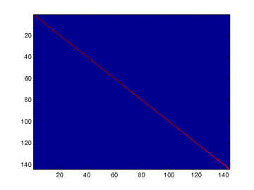
Step 4b: Check covariance
Similar to using PCA alone, PCA with whitening also results in processed data that has a diagonal covariance matrix. However, unlike PCA alone, whitening additionally ensures that the diagonal entries are equal to 1, i.e. that the covariance matrix is the identity matrix.
That would be the case if you were doing whitening alone with no regularization. However, in this case you are whitening with regularization, to avoid numerical/etc. problems associated with small eigenvalues. As a result of this, some of the diagonal entries of the covariance of your xPCAwhite will be smaller than 1.
To verify that your implementation of PCA whitening with and without regularization is correct, you can check these properties. Implement code to compute the covariance matrix and verify this property. (To check the result of PCA without whitening, simply set epsilon to 0, or close to 0, say 1e-10). As earlier, you can visualise the covariance matrix withimagesc. When visualised as an image, for PCA whitening without regularization you should see a red line across the diagonal (corresponding to the one entries) against a blue background (corresponding to the zero entries); for PCA whitening with regularization you should see a red line that slowly turns blue across the diagonal (corresponding to the 1 entries slowly becoming smaller).
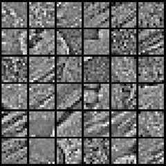
Step 5: ZCA whitening
Now implement ZCA whitening to produce the matrix xZCAWhite. VisualizexZCAWhite and compare it to the raw data,x. You should observe that whitening results in, among other things, enhanced edges. Try repeating this withepsilon set to 1, 0.1, and 0.01, and see what you obtain. The example shown below (left image) was obtained withepsilon = 0.1.
PCA |Whitening |Implementing PCA/Whitening | Exercise:PCA in 2D | Exercise:PCA and Whitening
- PCA Whitening ZCA Whitening
- Whitening&PCA
- PCA与Whitening
- pca 与 whitening
- PCA and Whitening Exercise
- PCA和whitening
- PCA, PCA whitening and ZCA whitening in 2D
- UFLDL Tutorial_Preprocessing: PCA and Whitening
- UFLDL Exercise:PCA and Whitening
- UFLDL Exercise:PCA and Whitening
- UFLDL Exercise:PCA and Whitening
- PCA详细讲解、ZCA、 Whitening
- UFLDL练习(PCA and Whitening && Softmax Regression)
- PCA ZCA Whitening on natural images
- 【Deep Learning】2、Preprocessing: PCA and Whitening
- Deep learning:十(PCA和whitening)
- PCA and Whitening编程代码整理
- Exercise:PCA and Whitening 代码示例
- VS 2010智能提示没有了
- apache如何开启gzip为VPS加速
- 邮箱下拉自动填充选择
- ACM-DFS之Accepted Necklace——hdu2660
- 使用Log4j为项目配置日志输出应用详细总结及示例演示.
- Whitening&PCA
- 黑马程序员--常用的正则表达式
- Linux设备驱动程序学习(2)-调试技术
- Linux查看进程的内存占用情况
- 多线程同步说明
- Spring Annotation 详解
- sc命令行添加windows服务
- 一个网友分享的成长经历
- 模块加载时 insmod “Invalid module format ”问题解决