相似图片搜索的原理

原文请参考：http://www.ruanyifeng.com/blog/2011/07/principle_of_similar_image_search.html

上个月，Google把"相似图片搜索"正式放上了首页。

你可以用一张图片，搜索互联网上所有与它相似的图片。点击搜索框中照相机的图标。

一个对话框会出现。

你输入网片的网址，或者直接上传图片，Google就会找出与其相似的图片。下面这张图片是美国女演员Alyson Hannigan。

上传后，Google返回如下结果：

类似的"相似图片搜索引擎"还有不少，TinEye甚至可以找出照片的拍摄背景。

==========================================================

这种技术的原理是什么？计算机怎么知道两张图片相似呢？

根据Neal Krawetz博士的解释，原理非常简单易懂。我们可以用一个快速算法，就达到基本的效果。

这里的关键技术叫做"感知哈希算法"（Perceptual hash algorithm），它的作用是对每张图片生成一个"指纹"（fingerprint）字符串，然后比较不同图片的指纹。结果越接近，就说明图片越相似。

下面是一个最简单的实现：

第一步，缩小尺寸。

将图片缩小到8x8的尺寸，总共64个像素。这一步的作用是去除图片的细节，只保留结构、明暗等基本信息，摒弃不同尺寸、比例带来的图片差异。

第二步，简化色彩。

将缩小后的图片，转为64级灰度。也就是说，所有像素点总共只有64种颜色。

第三步，计算平均值。

计算所有64个像素的灰度平均值。

第四步，比较像素的灰度。

将每个像素的灰度，与平均值进行比较。大于或等于平均值，记为1；小于平均值，记为0。

第五步，计算哈希值。

将上一步的比较结果，组合在一起，就构成了一个64位的整数，这就是这张图片的指纹。组合的次序并不重要，只要保证所有图片都采用同样次序就行了。

= = 8f373714acfcf4d0

得到指纹以后，就可以对比不同的图片，看看64位中有多少位是不一样的。在理论上，这等同于计算"汉明距离"（Hamming distance）。如果不相同的数据位不超过5，就说明两张图片很相似；如果大于10，就说明这是两张不同的图片。

具体的代码实现，可以参见Wote用python语言写的imgHash.py。代码很短，只有53行。使用的时候，第一个参数是基准图片，第二个参数是用来比较的其他图片所在的目录，返回结果是两张图片之间不相同的数据位数量（汉明距离）。

这种算法的优点是简单快速，不受图片大小缩放的影响，缺点是图片的内容不能变更。如果在图片上加几个文字，它就认不出来了。所以，它的最佳用途是根据缩略图，找出原图。

实际应用中，往往采用更强大的pHash算法和SIFT算法，它们能够识别图片的变形。只要变形程度不超过25%，它们就能匹配原图。这些算法虽然更复杂，但是原理与上面的简便算法是一样的，就是先将图片转化成Hash字符串，然后再进行比较。

未完待续....

原文请参考：http://www.ruanyifeng.com/blog/2013/03/similar_image_search_part_ii.html

二年前，我写了《相似图片搜索的原理》，介绍了一种最简单的实现方法。

昨天，我在isnowfy的网站看到，还有其他两种方法也很简单，这里做一些笔记。

一、颜色分布法

每张图片都可以生成颜色分布的直方图（color histogram）。如果两张图片的直方图很接近，就可以认为它们很相似。

任何一种颜色都是由红绿蓝三原色（RGB）构成的，所以上图共有4张直方图（三原色直方图 + 最后合成的直方图）。

如果每种原色都可以取256个值，那么整个颜色空间共有1600万种颜色（256的三次方）。针对这1600万种颜色比较直方图，计算量实在太大了，因此需要采用简化方法。可以将0～255分成四个区：0～63为第0区，64～127为第1区，128～191为第2区，192～255为第3区。这意味着红绿蓝分别有4个区，总共可以构成64种组合（4的3次方）。

任何一种颜色必然属于这64种组合中的一种，这样就可以统计每一种组合包含的像素数量。

上图是某张图片的颜色分布表，将表中最后一栏提取出来，组成一个64维向量(7414, 230, 0, 0, 8, ..., 109, 0, 0, 3415, 53929)。这个向量就是这张图片的特征值或者叫"指纹"。

于是，寻找相似图片就变成了找出与其最相似的向量。这可以用皮尔逊相关系数或者余弦相似度算出。

二、内容特征法

除了颜色构成，还可以从比较图片内容的相似性入手。

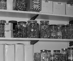
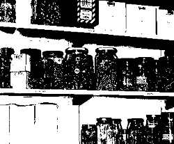
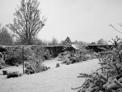
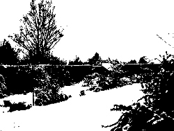
首先，将原图转成一张较小的灰度图片，假定为50x50像素。然后，确定一个阈值，将灰度图片转成黑白图片。

如果两张图片很相似，它们的黑白轮廓应该是相近的。于是，问题就变成了，第一步如何确定一个合理的阈值，正确呈现照片中的轮廓？

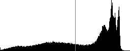
显然，前景色与背景色反差越大，轮廓就越明显。这意味着，如果我们找到一个值，可以使得前景色和背景色各自的"类内差异最小"（minimizing the intra-class variance），或者"类间差异最大"（maximizing the inter-class variance），那么这个值就是理想的阈值。

1979年，日本学者大津展之证明了，"类内差异最小"与"类间差异最大"是同一件事，即对应同一个阈值。他提出一种简单的算法，可以求出这个阈值，这被称为"大津法"（Otsu's method）。下面就是他的计算方法。

假定一张图片共有n个像素，其中灰度值小于阈值的像素为 n1 个，大于等于阈值的像素为 n2 个（ n1 + n2 = n ）。w1 和 w2 表示这两种像素各自的比重。

　　w1 = n1 / n

　　w2 = n2 / n

再假定，所有灰度值小于阈值的像素的平均值和方差分别为 μ1 和 σ1，所有灰度值大于等于阈值的像素的平均值和方差分别为 μ2 和 σ2。于是，可以得到

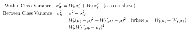
　　类内差异 = w1(σ1的平方) + w2(σ2的平方)

　　类间差异 = w1w2(μ1-μ2)^2

可以证明，这两个式子是等价的：得到"类内差异"的最小值，等同于得到"类间差异"的最大值。不过，从计算难度看，后者的计算要容易一些。

下一步用"穷举法"，将阈值从灰度的最低值到最高值，依次取一遍，分别代入上面的算式。使得"类内差异最小"或"类间差异最大"的那个值，就是最终的阈值。具体的实例和Java算法，后面会有展示

有了50x50像素的黑白缩略图，就等于有了一个50x50的0-1矩阵。矩阵的每个值对应原图的一个像素，0表示黑色，1表示白色。这个矩阵就是一张图片的特征矩阵。

两个特征矩阵的不同之处越少，就代表两张图片越相似。这可以用"异或运算"实现（即两个值之中只有一个为1，则运算结果为1，否则运算结果为0）。对不同图片的特征矩阵进行"异或运算"，结果中的1越少，就是越相似的图片。

具体的实例和Java算法: 原文地址http://www.labbookpages.co.uk/software/imgProc/otsuThreshold.html

Otsu Thresholding

Converting a greyscale image to monochrome is a common image processing task. Otsu's method,named after its inventor Nobuyuki Otsu, is one of many binarization algorithms. This page describeshow the algorithm works and provides a Java implementation, which can be easily ported to otherlanguages. If you are in a hurry, jump to the code.

• Otsu Thresholding Explained
• A Faster Approach
• Java Implementation
• Examples

Many thanks to Eric Moyer who spotted a potential overflow when two integers are multiplied inthe variance calculation. The example code has been updated with the integers cast to floats duringthe calculation.

---

Otsu Thresholding Explained

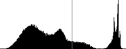
Otsu's thresholding method involves iterating through all the possible threshold values andcalculating a measure of spread for the pixel levels each side of the threshold, i.e. the pixelsthat either fall in foreground or background. The aim is to find the threshold value where the sumof foreground and background spreads is at its minimum.

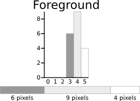
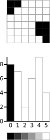
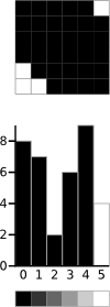
The algorithm will be demonstrated using the simple 6x6 image shown below. The histogram for theimage is shown next to it. To simplify the explanation, only 6 greyscale levels are used.

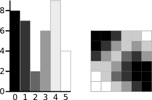
A 6-level greyscale image and its histogram

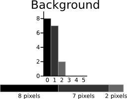
The calculations for finding the foreground and background variances (the measure of spread) fora single threshold are now shown. In this case the threshold value is 3.

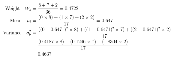
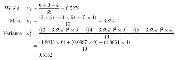
The next step is to calculate the 'Within-Class Variance'. This is simply the sum of thetwo variances multiplied by their associated weights.

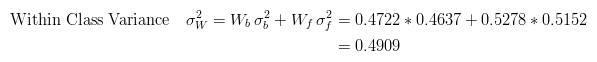
This final value is the 'sum of weighted variances' for the threshold value 3. This samecalculation needs to be performed for all the possible threshold values 0 to 5. The table belowshows the results for these calculations. The highlighted column shows the values for the thresholdcalculated above.

ThresholdT=0T=1T=2T=3T=4T=5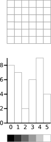 

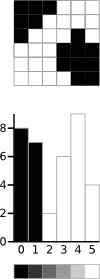
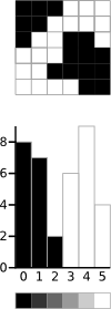
Weight, BackgroundWb = 0Wb = 0.222Wb = 0.4167Wb = 0.4722Wb = 0.6389Wb = 0.8889Mean, BackgroundMb = 0Mb = 0Mb = 0.4667Mb = 0.6471Mb = 1.2609Mb = 2.0313Variance, Backgroundσ2b = 0σ2b = 0σ2b = 0.2489σ2b = 0.4637σ2b = 1.4102σ2b = 2.5303 Weight, ForegroundWf = 1Wf = 0.7778Wf = 0.5833Wf = 0.5278Wf = 0.3611Wf = 0.1111Mean, ForegroundMf = 2.3611Mf = 3.0357Mf = 3.7143Mf = 3.8947Mf = 4.3077Mf = 5.000Variance, Foregroundσ2f = 3.1196σ2f = 1.9639σ2f = 0.7755σ2f = 0.5152σ2f = 0.2130σ2f = 0 Within Class Varianceσ2W = 3.1196σ2W = 1.5268σ2W = 0.5561σ2W = 0.4909σ2W = 0.9779σ2W = 2.2491

It can be seen that for the threshold equal to 3, as well as being used for the example, also has thelowest sum of weighted variances. Therefore, this is the final selected threshold. All pixels with a levelless than 3 are background, all those with a level equal to or greater than 3 are foreground. As theimages in the table show, this threshold works well.

Result of Otsu's Method

This approach for calculating Otsu's threshold is useful for explaining the theory, but it iscomputationally intensive, especially if you have a full 8-bit greyscale. The next section shows afaster method of performing the calculations which is much more appropriate for implementations.

---

A Faster Approach

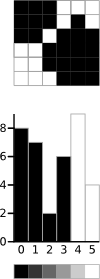
By a bit of manipulation, you can calculate what is called the between class variance,which is far quicker to calculate. Luckily, the threshold with the maximumbetween classvariance also has the minimum within class variance. So it can also be used for finding thebest threshold and therefore due to being simpler is a much better approach to use.

The table below shows the different variances for each threshold value.

ThresholdT=0T=1T=2T=3T=4T=5 Within Class Varianceσ2W = 3.1196σ2W = 1.5268σ2W = 0.5561σ2W = 0.4909σ2W = 0.9779σ2W = 2.2491Between Class Varianceσ2B = 0σ2B = 1.5928σ2B = 2.5635σ2B = 2.6287σ2B = 2.1417σ2B = 0.8705

---

Java Implementation

A simple demo program that uses the Otsu threshold is linked to below.

Otsu Threshold Demo

The important part of the algorithm is shown here. The input is an array of bytes,srcData that stores thegreyscale image.

File Excerpt: OtsuThresholder.java

// Calculate histogramint ptr = 0;while (ptr < srcData.length) {   int h = 0xFF & srcData[ptr];   histData[h] ++;   ptr ++;}// Total number of pixelsint total = srcData.length;float sum = 0;for (int t=0 ; t<256 ; t++) sum += t * histData[t];float sumB = 0;int wB = 0;int wF = 0;float varMax = 0;threshold = 0;for (int t=0 ; t<256 ; t++) {   wB += histData[t];               // Weight Background   if (wB == 0) continue;   wF = total - wB;                 // Weight Foreground   if (wF == 0) break;   sumB += (float) (t * histData[t]);   float mB = sumB / wB;            // Mean Background   float mF = (sum - sumB) / wF;    // Mean Foreground   // Calculate Between Class Variance   float varBetween = (float)wB * (float)wF * (mB - mF) * (mB - mF);   // Check if new maximum found   if (varBetween > varMax) {      varMax = varBetween;      threshold = t;   }}

---

Examples

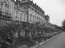
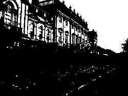
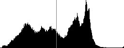
Here are a number of examples of the Otsu Method in use. It works well with images that have abi-modal histogram (those with two distinct regions).

Greyscale ImageBinary ImageHistogram