Singular value decomposition
来源:互联网 发布:python算法书籍 编辑:程序博客网 时间:2024/05/20 06:27
矩阵分解 (decomposition, factorization)是将矩阵拆解为数个矩阵的乘积,可分为三角分解、满秩分解、QR分解、Jordan分解和SVD(奇异值)分解等,常见的有三种:1)三角分解法 (Triangular Factorization),2)QR 分解法 (QR Factorization),3)奇异值分解法 (Singular Value Decompostion)。
(1) 三角分解法
三角分解法是将原正方 (square) 矩阵分解成一个上三角形矩阵 或是排列(permuted) 的上三角形矩阵和一个 下三角形矩阵,这样的分解法又称为LU分解法。它的用途主要在简化一个大矩阵的行列式值的计算过程,求 反矩阵,和求解联立方程组。不过要注意这种分解法所得到的上下三角形矩阵并非唯一,还可找到数个不同 的一对上下三角形矩阵,此两三角形矩阵相乘也会得到原矩阵。
MATLAB以lu函数来执行lu分解法, 其语法为[L,U]=lu(A)。
(2) QR分解法
QR分解法是将矩阵分解成一个正规正交矩阵与上三角形矩阵,所以称为QR分解法,与此正规正交矩阵的通用符号Q有关。
MATLAB以qr函数来执行QR分解法, 其语法为[Q,R]=qr(A)。
(3) 奇异值分解法
奇异值分解 (singular value decomposition,SVD) 是另一种正交矩阵分解法;SVD是最可靠的分解法,但是它比QR 分解法要花上近十倍的计算时间。[U,S,V]=svd(A),其中U和V代表二个相互正交矩阵,而S代表一对角矩阵。 和QR分解法相同者, 原矩阵A不必为正方矩阵。使用SVD分解法的用途是解最小平方误差法和数据压缩。
MATLAB以svd函数来执行svd分解法, 其语法为[S,V,D]=svd(A)。
Singular value decomposition

In linear algebra, the singular value decomposition (SVD) is afactorization of a real or complex matrix, with many useful applications in signal processing and statistics.
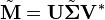
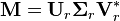
Formally, the singular value decomposition of anm×n real or complex matrix M is a factorization of the form
where U is am×m real or complex unitary matrix, Σ is an m×n rectangular diagonal matrix with nonnegative real numbers on the diagonal, andV* (the conjugate transpose of V, or simply the transpose of V if V is real) is an n×n real or complex unitary matrix. The diagonal entries Σi,i of Σ are known as thesingular values ofM. The m columns of U and the n columns of V are called the left-singular vectors and right-singular vectors ofM, respectively.
The singular value decomposition and theeigendecomposition are closely related. Namely:
- The left-singular vectors ofM are eigenvectors of MM*.
- The right-singular vectors ofM are eigenvectors of M*M.
- The non-zero singular values ofM (found on the diagonal entries of Σ) are the square roots of the non-zeroeigenvalues of both M*M and MM*.
Applications which employ the SVD include computing thepseudoinverse, least squares fitting of data, matrix approximation, and determining the rank, range and null space of a matrix.
Contents
- 1Statement of the theorem
- 2Intuitive interpretations
- 3Example
- 4Singular values, singular vectors, and their relation to the SVD
- 5Applications of the SVD
- 6Relation to eigenvalue decomposition
- 7Existence
- 8Geometric meaning
- 9Calculating the SVD
- 10Reduced SVDs
- 11Norms
- 12Tensor SVD
- 13Bounded operators on Hilbert spaces
- 14History
- 15See also
- 16Notes
- 17References
Statement of the theorem
Suppose M is anm×n matrix whose entries come from the field K, which is either the field of real numbers or the field of complex numbers. Then there exists a factorization of the form
where U is anm×m unitary matrix (orthogonal matrix if "K" is real) overK, the matrix Σ is an m×n diagonal matrix with nonnegative real numbers on the diagonal, and the n×n unitary matrixV* denotes the conjugate transpose of the n×n unitary matrix V. Such a factorization is called a singular value decomposition ofM.
The diagonal entries of Σ are known as thesingular values ofM. A common convention is to list the singular values in descending order. In this case, the diagonal matrix Σ is uniquely determined byM (though the matrices U and V are not).
Intuitive interpretations
Rotation, scaling
In the special but common case in which M is just anm×m square matrix with positive determinant whose entries are plain real numbers, then U, V*, and Σ are m×m matrices of real numbers as well, Σ can be regarded as ascaling matrix, and U and V* can be viewed as rotation matrices.
If the above mentioned conditions are met, the expression can thus be intuitively interpreted as acomposition (or sequence) of three geometrical transformations: a rotation, a scaling, and another rotation. For instance, the figure above explains how a shear matrix can be described as such a sequence.
Singular values as semiaxes of an ellipse or ellipsoid
As shown in the figure, thesingular values can be interpreted as the semiaxes of an ellipse in 2D. This concept can be generalized to n-dimensional Euclidean space, with the singular values of any n×n square matrix being viewed as the semiaxes of an n-dimensional ellipsoid. See below for further details.
The columns ofU and V are orthonormal bases
Since U andV* are unitary, the columns of each of them form a set of orthonormal vectors, which can be regarded as basis vectors. By the definition of a unitary matrix, the same is true for their conjugate transposesU* and V. In short, the columns of U, U*, V, and V* are orthonormal bases.
Example
Consider the 4×5 matrix
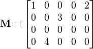
A singular value decomposition of this matrix is given by
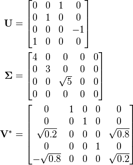
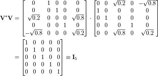
Notice  is zero outside of the diagonal and one diagonal element is zero. Furthermore, because the matrices
  and
and areunitary, multiplying by their respective conjugate transposes yields identity matrices, as shown below. In this case, because and are real valued, they each are anorthogonal matrix.

and
This particular singular value decomposition is not unique. Choosing such that

is also a valid singular value decomposition.
Singular values, singular vectors, and their relation to the SVD
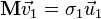
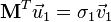
A non-negative real number σ is asingular value forM if and only if there exist unit-length vectors u in Km andv in Kn such that

The vectors u andv are called left-singular and right-singular vectors for σ, respectively.
In any singular value decomposition
the diagonal entries of Σ are equal to the singular values ofM. The columns of U and V are, respectively, left- and right-singular vectors for the corresponding singular values. Consequently, the above theorem implies that:
- An m × n matrix M has at most p = min(m,n) distinct singular values.
- It is always possible to find anorthogonal basis U for Km consisting of left-singular vectors ofM.
- It is always possible to find an orthogonal basisV for Kn consisting of right-singular vectors ofM.
A singular value for which we can find two left (or right) singular vectors that are linearly independent is calleddegenerate.
Non-degenerate singular values always have unique left- and right-singular vectors, up to multiplication by a unit-phase factoreiφ (for the real case up to sign). Consequently, if all singular values ofM are non-degenerate and non-zero, then its singular value decomposition is unique, up to multiplication of a column ofU by a unit-phase factor and simultaneous multiplication of the corresponding column ofV by the same unit-phase factor.
Degenerate singular values, by definition, have non-unique singular vectors. Furthermore, ifu1 and u2 are two left-singular vectors which both correspond to the singular value σ, then any normalized linear combination of the two vectors is also a left-singular vector corresponding to the singular value σ. The similar statement is true for right-singular vectors. Consequently, if M has degenerate singular values, then its singular value decomposition is not unique.
Applications of the SVD
Pseudoinverse
The singular value decomposition can be used for computing thepseudoinverse of a matrix. Indeed, the pseudoinverse of the matrix M with singular value decomposition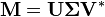 is
is

where Σ+ is the pseudoinverse of Σ, which is formed by replacing every non-zero diagonal entry by itsreciprocal and transposing the resulting matrix. The pseudoinverse is one way to solvelinear least squares problems.
Solving homogeneous linear equations
A set of homogeneous linear equations can be written as  for a matrix
 and vector
 . A typical situation is that is known and a non-zero is to be determined which satisfies the equation. Such an belongs to'snull space and is sometimes called a (right) null vector of . The vector can be characterized as a right-singular vector corresponding to a singular value of that is zero. This observation means that if is asquare matrix and has no vanishing singular value, the equation has no non-zero as a solution. It also means that if there are several vanishing singular values, any linear combination of the corresponding right-singular vectors is a valid solution. Analogously to the definition of a (right) null vector, a non-zero satisfying
 , with
 denoting the conjugate transpose of, is called a left null vector of.
Total least squares minimization
A total least squares problem refers to determining the vector  which minimizes the2-norm of a vector
  under the constraint
 . The solution turns out to be the right-singular vector of corresponding to the smallest singular value.
Range, null space and rank
Another application of the SVD is that it provides an explicit representation of therange and null space of a matrix M. The right-singular vectors corresponding to vanishing singular values ofM span the null space of M. E.g., the null space is spanned by the last two columns of in the above example. The left-singular vectors corresponding to the non-zero singular values ofM span the range of M. As a consequence, the rank of M equals the number of non-zero singular values which is the same as the number of non-zero diagonal elements in.
In numerical linear algebra the singular values can be used to determine theeffective rank of a matrix, as rounding error may lead to small but non-zero singular values in a rank deficient matrix.
Low-rank matrix approximation
Some practical applications need to solve the problem of approximating a matrix with another matrix
 , saidtruncated, which has a specific rank
  . In the case that the approximation is based on minimizing theFrobenius norm of the difference between and under the constraint that
 it turns out that the solution is given by the SVD of, namely
where  is the same matrix as except that it contains only the largest singular values (the other singular values are replaced by zero). This is known as theEckart–Young theorem, as it was proved by those two authors in 1936 (although it was later found to have been known to earlier authors; seeStewart 1993).
Separable models
The SVD can be thought of as decomposing a matrix into a weighted, ordered sum of separable matrices. By separable, we mean that a matrix can be written as anouter product of two vectors  , or, in coordinates,
 . Specifically, the matrix M can be decomposed as:
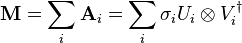
Here  and
and are theith columns of the corresponding SVD matrices, are the ordered singular values, and each
 is separable. The SVD can be used to find the decomposition of an image processing filter into separable horizontal and vertical filters. Note that the number of non-zero is exactly the rank of the matrix.
Separable models often arise in biological systems, and the SVD decomposition is useful to analyze such systems. For example, some visual area V1 simple cells' receptive fields can be well described[1] by a Gabor filter in the space domain multiplied by a modulation function in the time domain. Thus, given a linear filter evaluated through, for example,reverse correlation, one can rearrange the two spatial dimensions into one dimension, thus yielding a two-dimensional filter (space, time) which can be decomposed through SVD. The first column of U in the SVD decomposition is then a Gabor while the first column of V represents the time modulation (or vice-versa). One may then define an index of separability, , which is the fraction of the power in the matrix M which is accounted for by the first separable matrix in the decomposition.[2]
Nearest orthogonal matrix
It is possible to use the SVD of to determine theorthogonal matrix  closest to. The closeness of fit is measured by theFrobenius norm of
  . The solution is the product
 .[3] This intuitively makes sense because an orthogonal matrix would have the decomposition
 where
where is the identity matrix, so that if
 then the product
 amounts to replacing the singular values with ones.
A similar problem, with interesting applications inshape analysis, is the orthogonal Procrustes problem, which consists of finding an orthogonal matrix which most closely maps to . Specifically,

where  denotes the Frobenius norm.
This problem is equivalent to finding the nearest orthogonal matrix to a given matrix .
.
The Kabsch algorithm
The Kabsch algorithm (called Wahba's problem in other fields) uses SVD to compute the optimal rotation (with respect to least-squares minimization) that will align a set of points with a corresponding set of points. It is used, among other applications, to compare the structures of molecules.
Signal processing
The SVD and pseudoinverse have been successfully applied to signal processing and big data, e.g., in genomic signal processing.[4][5][6][7]
Other examples
The SVD is also applied extensively to the study of linearinverse problems, and is useful in the analysis of regularization methods such as that ofTikhonov. It is widely used in statistics where it is related to principal component analysis and to Correspondence analysis, and in signal processing and pattern recognition. It is also used in output-only modal analysis, where the non-scaled mode shapes can be determined from the singular vectors. Yet another usage islatent semantic indexing in natural language text processing.
The SVD also plays a crucial role in the field ofquantum information, in a form often referred to as the Schmidt decomposition. Through it, states of two quantum systems are naturally decomposed, providing a necessary and sufficient condition for them to beentangled: if the rank of the  matrix is larger than one.
One application of SVD to rather large matrices is innumerical weather prediction, where Lanczos methods are used to estimate the most linearly quickly growing few perturbations to the central numerical weather prediction over a given initial forward time period; i.e., the singular vectors corresponding to the largest singular values of the linearized propagator for the global weather over that time interval. The output singular vectors in this case are entire weather systems. These perturbations are then run through the full nonlinear model to generate anensemble forecast, giving a handle on some of the uncertainty that should be allowed for around the current central prediction.
Another application of SVD for daily life is that point in perspective view can be unprojected in a photo using the calculated SVD matrix, this application leads to measuring length (a.k.a. the distance of two unprojected points in perspective photo) by marking out the 4 corner points of known-size object in a single photo. PRuler is a demo to implement this application by taking a photo of a regular credit card.
SVD has also been applied to reduced order modelling. The aim of reduced order modelling is to reduce the number of degrees of freedom in a complex system which is to be modelled. SVD was coupled with radial basis functions to interpolate solutions to three-dimensional unsteady flow problems.[8]
SVD has also been applied in inverse problem theory. An important application is constructing computational models of oil reservoirs.[9]
Singular value decomposition is used inrecommender systems to predict people's item ratings.[10]
Relation to eigenvalue decomposition
The singular value decomposition is very general in the sense that it can be applied to anym × n matrix whereas eigenvalue decomposition can only be applied to certain classes of square matrices. Nevertheless, the two decompositions are related.
Given an SVD of M, as described above, the following two relations hold:
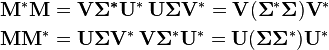
The right-hand sides of these relations describe the eigenvalue decompositions of the left-hand sides. Consequently:
- The columns of V (right-singular vectors) are eigenvectors of
 .
. - The columns of U (left-singular vectors) are eigenvectors of
 .
. - The non-zero elements ofΣ (non-zero singular values) are the square roots of the non-zero eigenvalues of or.
- The columns of V (right-singular vectors) are eigenvectors of
In the special case thatM is a normal matrix, which by definition must be square, the spectral theorem says that it can be unitarily diagonalized using a basis of eigenvectors, so that it can be written 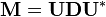 for a unitary matrixU and a diagonal matrix D. When M is also positive semi-definite, the decomposition is also a singular value decomposition.
However, the eigenvalue decomposition and the singular value decomposition differ for all other matricesM: the eigenvalue decomposition is 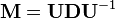 whereU is not necessarily unitary and D is not necessarily positive semi-definite, while the SVD is whereΣ is a diagonal positive semi-definite, and U and V are unitary matrices that are not necessarily related except through the matrixM.
Existence
An eigenvalue λ of a matrixM is characterized by the algebraic relation M u = λ u. WhenM is Hermitian, a variational characterization is also available. Let M be a realn × n symmetric matrix. Define f:Rn →R by f(x) = xT M x. By theextreme value theorem, this continuous function attains a maximum at some u when restricted to the closed unit sphere {||x|| ≤ 1}. By the Lagrange multipliers theorem, u necessarily satisfies

where the nabla symbol, , is thedel operator.
A short calculation shows the above leads toM u = λ u (symmetry of M is needed here). Therefore λ is the largest eigenvalue of M. The same calculation performed on the orthogonal complement ofu gives the next largest eigenvalue and so on. The complex Hermitian case is similar; theref(x) = x* M x is a real-valued function of 2n real variables.
Singular values are similar in that they can be described algebraically or from variational principles. Although, unlike the eigenvalue case, Hermiticity, or symmetry, ofM is no longer required.
This section gives these two arguments for existence of singular value decomposition.
Based on the spectral theorem
Let M be anm-by-n matrix with complex entries. M*M is positive semidefinite and Hermitian. By thespectral theorem, there exists a unitary n-by-n matrix V such that
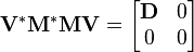
where D is diagonal and positive definite. PartitionV appropriately so we can write

Therefore V1*M*MV1 =D and V2*M*MV2 = 0. The latter meansMV2 = 0.
Also, since V is unitary,V1*V1 = I, V2*V2 =I and V1V1* + V2V2* =I.
Define
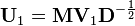
Then

We see that this is almost the desired result, except thatU1 and V1 are not unitary in general, but merelyisometries. To finish the argument, one simply has to "fill out" these matrices to obtain unitaries. For example, one can chooseU2 such that
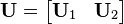
is unitary.
Define
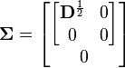
where extra zero rows are addedor removed to make the number of zero rows equal the number of columns ofU2. Then
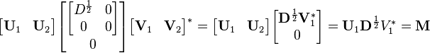
which is the desired result:
Notice the argument could begin with diagonalizingMM* rather than M*M (This shows directly that MM* and M*M have the same non-zero eigenvalues).
Based on variational characterization
The singular values can also be characterized as the maxima ofuTMv, considered as a function of u and v, over particular subspaces. The singular vectors are the values of u andv where these maxima are attained.
Let M denote anm × n matrix with real entries. Let  and
and denote the sets of unit 2-norm vectors inRm and Rn respectively. Define the function
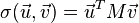
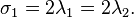
for vectors u ∈ andv ∈ . Consider the functionσ restricted to ×. Since both and arecompact sets, their product is also compact. Furthermore, since σ is continuous, it attains a largest value for at least one pair of vectorsu ∈ andv ∈ . This largest value is denotedσ1 and the corresponding vectors are denoted u1 andv1. Since  is the largest value of
 it must be non-negative. If it were negative, changing the sign of eitheru1 or v1 would make it positive and therefore larger.
Statement:u1, v1 are left and right-singular vectors ofM with corresponding singular value σ1.
Proof: Similar to the eigenvalues case, by assumption the two vectors satisfy the Lagrange multiplier equation:

After some algebra, this becomes
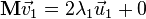
and
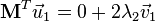
Multiplying the first equation from left by and the second equation from left by
 and taking ||u|| = ||v|| = 1 into account gives
Plugging this into the pair of equations above, we have
and
This proves the statement.
More singular vectors and singular values can be found by maximizingσ(u, v) over normalized u, v which are orthogonal tou1 and v1, respectively.
The passage from real to complex is similar to the eigenvalue case.
Geometric meaning
Because U andV are unitary, we know that the columns u1, …, um ofU yield an orthonormal basis of Km and the columns v1, …,vn of V yield an orthonormal basis of Kn (with respect to the standardscalar products on these spaces).
The linear transformation T :Kn → Km that takes a vectorx to Mx has a particularly simple description with respect to these orthonormal bases: we haveT(vi) = σi ui, for i = 1,...,min(m,n), where σi is the i-th diagonal entry of Σ, and T(vi) = 0 fori > min(m,n).
The geometric content of the SVD theorem can thus be summarized as follows: for every linear mapT :Kn → Km one can find orthonormal bases ofKn and Km such that T maps the i-th basis vector of Kn to a non-negative multiple of thei-th basis vector of Km, and sends the left-over basis vectors to zero. With respect to these bases, the mapT is therefore represented by a diagonal matrix with non-negative real diagonal entries.
To get a more visual flavour of singular values and SVD decomposition —at least when working on real vector spaces— consider the sphereS of radius one in Rn. The linear mapT maps this sphere onto an ellipsoid in Rm. Non-zero singular values are simply the lengths of thesemi-axes of this ellipsoid. Especially when n=m, and all the singular values are distinct and non-zero, the SVD of the linear mapT can be easily analysed as a succession of three consecutive moves : consider the ellipsoidT(S) and specifically its axes ; then consider the directions inRn sent by T onto these axes. These directions happen to be mutually orthogonal. Apply first an isometryv* sending these directions to the coordinate axes of Rn. On a second move, apply anendomorphism d diagonalized along the coordinate axes and stretching or shrinking in each direction, using the semi-axes lengths ofT(S) as stretching coefficients. The composition d o v* then sends the unit-sphere onto an ellipsoid isometric to T(S). To define the third and last moveu, apply an isometry to this ellipsoid so as to carry it over T(S). As can be easily checked, the compositionu o d o v* coincides with T.
Calculating the SVD
Numerical approach
The SVD of a matrix M is typically computed by a two-step procedure. In the first step, the matrix is reduced to abidiagonal matrix. This takes O(mn2) floating-point operations (flops), assuming that m ≥ n. The second step is to compute the SVD of the bidiagonal matrix. This step can only be done with aniterative method (as with eigenvalue algorithms). However, in practice it suffices to compute the SVD up to a certain precision, like themachine epsilon. If this precision is considered constant, then the second step takes O(n) iterations, each costing O(n) flops. Thus, the first step is more expensive, and the overall cost is O(mn2) flops (Trefethen & Bau III 1997, Lecture 31).
The first step can be done usingHouseholder reflections for a cost of 4mn2 − 4n3/3 flops, assuming that only the singular values are needed and not the singular vectors. Ifm is much larger than n then it is advantageous to first reduce the matrixM to a triangular matrix with the QR decomposition and then use Householder reflections to further reduce the matrix to bidiagonal form; the combined cost is 2mn2 + 2n3 flops (Trefethen & Bau III 1997, Lecture 31).
The second step can be done by a variant of theQR algorithm for the computation of eigenvalues, which was first described byGolub & Kahan (1965). The LAPACK subroutine DBDSQR[11] implements this iterative method, with some modifications to cover the case where the singular values are very small (Demmel & Kahan 1990). Together with a first step using Householder reflections and, if appropriate, QR decomposition, this forms the DGESVD[12] routine for the computation of the singular value decomposition.
The same algorithm is implemented in theGNU Scientific Library (GSL). The GSL also offers an alternative method, which uses a one-sidedJacobi orthogonalization in step 2 (GSL Team 2007). This method computes the SVD of the bidiagonal matrix by solving a sequence of 2-by-2 SVD problems, similar to how the Jacobi eigenvalue algorithm solves a sequence of 2-by-2 eigenvalue methods (Golub & Van Loan 1996, §8.6.3). Yet another method for step 2 uses the idea of divide-and-conquer eigenvalue algorithms (Trefethen & Bau III 1997, Lecture 31).
Analytic result of 2-by-2 SVD
The singular values of a 2-by-2 matrix can be found analytically. Let the matrix be
where  are complex numbers that parameterize the matrix, is the identity matrix, and denote thePauli matrices. Then its two singular values are given by

Reduced SVDs
In applications it is quite unusual for the full SVD, including a full unitary decomposition of the null-space of the matrix, to be required. Instead, it is often sufficient (as well as faster, and more economical for storage) to compute a reduced version of the SVD. The following can be distinguished for anm×n matrix M of rank r:
Thin SVD

Only the n column vectors ofU corresponding to the row vectors of V* are calculated. The remaining column vectors ofU are not calculated. This is significantly quicker and more economical than the full SVD ifn≪m. The matrix Un is thus m×n, Σn isn×n diagonal, and V is n×n.
The first stage in the calculation of a thin SVD will usually be aQR decomposition of M, which can make for a significantly quicker calculation ifn≪m.
Compact SVD
Only the r column vectors ofU and r row vectors of V* corresponding to the non-zero singular values Σr are calculated. The remaining vectors ofU and V* are not calculated. This is quicker and more economical than the thin SVD ifr≪n. The matrix Ur is thus m×r, Σr isr×r diagonal, and Vr* is r×n.
Truncated SVD

Only the t column vectors ofU and t row vectors of V* corresponding to the t largest singular values Σt are calculated. The rest of the matrix is discarded. This can be much quicker and more economical than the compact SVD ift≪r. The matrix Ut is thus m×t, Σt ist×t diagonal, and Vt* is t×n.
Of course the truncated SVD is no longer an exact decomposition of the original matrixM, but as discussed above, the approximate matrix is in a very useful sense the closest approximation toM that can be achieved by a matrix of rank t.
Norms
Ky Fan norms
The sum of the k largest singular values ofM is a matrix norm, the Ky Fan k-norm of M.
The first of the Ky Fan norms, the Ky Fan 1-norm is the same as theoperator norm of M as a linear operator with respect to the Euclidean norms ofKm and Kn. In other words, the Ky Fan 1-norm is the operator norm induced by the standardl2 Euclidean inner product. For this reason, it is also called the operator 2-norm. One can easily verify the relationship between the Ky Fan 1-norm and singular values. It is true in general, for a bounded operatorM on (possibly infinite-dimensional) Hilbert spaces
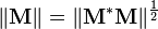
But, in the matrix case,M*M½ is a normal matrix, so ||M* M||½ is the largest eigenvalue of M* M½, i.e. the largest singular value of M.
The last of the Ky Fan norms, the sum of all singular values, is thetrace norm (also known as the 'nuclear norm'), defined by ||M|| = Tr[(M*M)½] (the eigenvalues ofM* M are the squares of the singular values).
Hilbert–Schmidt norm
The singular values are related to another norm on the space of operators. Consider theHilbert–Schmidt inner product on the n × n matrices, defined by . So the induced norm is
 . Since trace is invariant under unitary equivalence, this shows

where are the singular values ofM. This is called the Frobenius norm,Schatten 2-norm, or Hilbert–Schmidt norm of M. Direct calculation shows that if

the Frobenius norm ofM coincides with
Tensor SVD
The problem of finding a low rank approximation to a tensor is ill-posed. In other words, a best possible solution does not exist, but instead a sequence of better and better approximations that converge to infinitely large matrices. In spite of this, there are several ways to attempt decomposition.
Two types of tensor decompositions exist, which generalise SVD to multi-way arrays. One of them decomposes a tensor into a sum of rank-1 tensors, seeCandecomp-PARAFAC (CP) algorithm. The CP algorithm should not be confused with a rank-R decomposition but, for a givenN, it decomposes a tensor into a sum of N rank-1 tensors that optimally fit the original tensor. The second type of decomposition computes the orthonormal subspaces associated with the different axes or modes of a tensor (orthonormal row space, column space, fiber space, etc.). This decomposition is referred to in the literature as theTucker3/TuckerM, M-mode SVD, multilinear SVD and sometimes referred to as ahigher-order SVD (HOSVD). In addition, multilinear principal component analysis in multilinear subspace learning involves the same mathematical operations as Tucker decomposition, being used in a different context ofdimensionality reduction.
Bounded operators on Hilbert spaces
The factorization can be extended to a bounded operator M on a separable Hilbert space H. Namely, for any bounded operatorM, there exist a partial isometry U, a unitary V, a measure space (X, μ), and a non-negative measurablef such that
where  is themultiplication by f on L2(X, μ).
This can be shown by mimicking the linear algebraic argument for the matricial case above.VTf V* is the unique positive square root of M*M, as given by theBorel functional calculus for self adjoint operators. The reason why U need not be unitary is because, unlike the finite-dimensional case, given an isometryU1 with nontrivial kernel, a suitable U2 may not be found such that

is a unitary operator.
As for matrices, the singular value factorization is equivalent to thepolar decomposition for operators: we can simply write

and notice that U V* is still a partial isometry while VTf V* is positive.
Singular values and compact operators
To extend notion of singular values and left/right-singular vectors to the operator case, one needs to restrict tocompact operators. It is a general fact that compact operators on Banach spaces have only discrete spectrum. This is also true for compact operators on Hilbert spaces, sinceHilbert spaces are a special case of Banach spaces. If T is compact, every non-zeroλ in its spectrum is an eigenvalue. Furthermore, a compact self adjoint operator can be diagonalized by its eigenvectors. IfM is compact, so is M*M. Applying the diagonalization result, the unitary image of its positive square rootTf has a set of orthonormal eigenvectors {ei} corresponding to strictly positive eigenvalues {σi}. For any ψ ∈ H,

where the series converges in the norm topology onH. Notice how this resembles the expression from the finite-dimensional case. Theσi 's are called the singular values of M. {U ei} and {V ei} can be considered the left- and right-singular vectors ofM respectively.
Compact operators on a Hilbert space are the closure offinite-rank operators in the uniform operator topology. The above series expression gives an explicit such representation. An immediate consequence of this is:
TheoremM is compact if and only if M*M is compact.
History
The singular value decomposition was originally developed bydifferential geometers, who wished to determine whether a real bilinear form could be made equal to another by independent orthogonal transformations of the two spaces it acts on.Eugenio Beltrami and Camille Jordan discovered independently, in 1873 and 1874 respectively, that the singular values of the bilinear forms, represented as a matrix, form acomplete set of invariants for bilinear forms under orthogonal substitutions. James Joseph Sylvester also arrived at the singular value decomposition for real square matrices in 1889, apparently independently of both Beltrami and Jordan. Sylvester called the singular values thecanonical multipliers of the matrix A. The fourth mathematician to discover the singular value decomposition independently is Autonne in 1915, who arrived at it via thepolar decomposition. The first proof of the singular value decomposition for rectangular and complex matrices seems to be byCarl Eckart and Gale Young in 1936;[13] they saw it as a generalization of theprincipal axis[disambiguation needed] transformation for Hermitian matrices.
In 1907, Erhard Schmidt defined an analog of singular values for integral operators (which are compact, under some weak technical assumptions); it seems he was unaware of the parallel work on singular values of finite matrices. This theory was further developed byÉmile Picard in 1910, who is the first to call the numbers  singular values (or in French, valeurs singulières).
Practical methods for computing the SVD date back toKogbetliantz in 1954, 1955 and Hestenes in 1958.[14] resembling closely theJacobi eigenvalue algorithm, which uses plane rotations or Givens rotations. However, these were replaced by the method of Gene Golub and William Kahan published in 1965,[15] which usesHouseholder transformations or reflections. In 1970, Golub and Christian Reinsch[16] published a variant of the Golub/Kahan algorithm that is still the one most-used today.
See also
- Canonical correlation analysis (CCA)
- Canonical form
- Correspondence analysis (CA)
- Curse of dimensionality
- Digital signal processing
- Dimension reduction
- Eigendecomposition
- Empirical orthogonal functions (EOFs)
- Fourier analysis
- Fourier-related transforms
- Generalized singular value decomposition
- K-SVD
- Latent semantic analysis
- Latent semantic indexing
- Linear least squares
- Locality sensitive hashing
- Low-rank approximation
- Matrix decomposition
- Multilinear principal component analysis (MPCA)
- Nearest neighbor search
- Non-linear iterative partial least squares
- Polar decomposition
- Principal components analysis (PCA)
- Singular value
- Time series
- Two-dimensional singular value decomposition (2DSVD)
- von Neumann's trace inequality
- Wavelet compression
Notes
- DeAngelis GC, Ohzawa I, Freeman RD (October 1995)."Receptive-field dynamics in the central visual pathways". Trends Neurosci.18 (10): 451–8. doi:10.1016/0166-2236(95)94496-R.PMID 8545912.
- Depireux DA, Simon JZ, Klein DJ, Shamma SA (March 2001)."Spectro-temporal response field characterization with dynamic ripples in ferret primary auditory cortex".J. Neurophysiol. 85 (3): 1220–34. PMID 11247991.
- The Singular Value Decomposition in Symmetric (Lowdin) Orthogonalization and Data Compression
- O. Alter, P. O. Brown and D. Botstein (September 2000)."Singular Value Decomposition for Genome-Wide Expression Data Processing and Modeling".PNAS 97 (18): 10101–10106. doi:10.1073/pnas.97.18.10101.
- O. Alter and G. H. Golub (November 2004)."Integrative Analysis of Genome-Scale Data by Using Pseudoinverse Projection Predicts Novel Correlation Between DNA Replication and RNA Transcription".PNAS 101 (47): 16577–16582. doi:10.1073/pnas.0406767101.
- O. Alter and G. H. Golub (August 2006)."Singular Value Decomposition of Genome-Scale mRNA Lengths Distribution Reveals Asymmetry in RNA Gel Electrophoresis Band Broadening".PNAS 103 (32): 11828–11833. doi:10.1073/pnas.0604756103.
- N. M. Bertagnolli, J. A. Drake, J. M. Tennessen and O. Alter (November 2013)."SVD Identifies Transcript Length Distribution Functions from DNA Microarray Data and Reveals Evolutionary Forces Globally Affecting GBM Metabolism".PLoS One 8 (11): e78913. doi:10.1371/journal.pone.0078913.Highlight.
- S. Walton, , O. Hassan , K. Morgan, Reduced order modelling for unsteady fluid flow using proper orthogonal decomposition and radial basis functions, Applied Mathematical Modelling, http://www.sciencedirect.com/science/article/pii/S0307904X13002771
- Gharib Shirangi, M., History matching production data and uncertainty assessment with an efficient TSVD parameterization algorithm, Journal of Petroleum Science and Engineering, http://www.sciencedirect.com/science/article/pii/S0920410513003227
- Sarwar, Badrul; Karypis, George; Konstan, Joseph A. & Riedl, John T. (2000).Application of Dimensionality Reduction in Recommender System -- A Case Study (PDF).University of Minnesota. Retrieved May 26, 2014.
- Netlib.org
- Netlib.org
- Eckart, C.; Young, G. (1936). "The approximation of one matrix by another of lower rank".Psychometrika1 (3): 211–8. doi:10.1007/BF02288367.
- Hestenes, M. R. (1958). "Inversion of Matrices by Biorthogonalization and Related Results".Journal of the Society for Industrial and Applied Mathematics 6 (1): 51–90.doi:10.1137/0106005.JSTOR 2098862.MR 0092215.
- Golub, G. H.; Kahan, W. (1965). "Calculating the singular values and pseudo-inverse of a matrix".Journal of the Society for Industrial and Applied Mathematics: Series B, Numerical Analysis2 (2): 205–224. doi:10.1137/0702016.JSTOR 2949777.MR 0183105.
- Golub, G. H.; Reinsch, C. (1970). "Singular value decomposition and least squares solutions".Numerische Mathematik 14 (5): 403–420. doi:10.1007/BF02163027.MR 1553974.
References
- Trefethen, Lloyd N.; Bau III, David (1997).Numerical linear algebra. Philadelphia: Society for Industrial and Applied Mathematics.ISBN 978-0-89871-361-9.
- Demmel, James;Kahan, William (1990). "Accurate singular values of bidiagonal matrices". Society for Industrial and Applied Mathematics. Journal on Scientific and Statistical Computing11 (5): 873–912. doi:10.1137/0911052.
- Golub, Gene H.;Kahan, William (1965). "Calculating the singular values and pseudo-inverse of a matrix".Journal of the Society for Industrial and Applied Mathematics: Series B, Numerical Analysis2 (2): 205–224. doi:10.1137/0702016.JSTOR 2949777.
- Golub, Gene H.;Van Loan, Charles F. (1996). Matrix Computations (3rd ed.). Johns Hopkins.ISBN 978-0-8018-5414-9.
- GSL Team (2007)."§14.4 Singular Value Decomposition". GNU Scientific Library. Reference Manual.
- Halldor, Bjornsson and Venegas, Silvia A. (1997)."A manual for EOF and SVD analyses of climate data". McGill University, CCGCR Report No. 97-1, Montréal, Québec, 52pp.
- Hansen, P. C. (1987). "The truncated SVD as a method for regularization".BIT 27: 534–553. doi:10.1007/BF01937276.
- Horn, Roger A.; Johnson, Charles R. (1985). "Section 7.3".Matrix Analysis. Cambridge University Press. ISBN 0-521-38632-2.
- Horn, Roger A.; Johnson, Charles R. (1991). "Chapter 3".Topics in Matrix Analysis. Cambridge University Press. ISBN 0-521-46713-6.
- Samet, H. (2006).Foundations of Multidimensional and Metric Data Structures. Morgan Kaufmann.ISBN 0-12-369446-9.
- Strang G. (1998). "Section 6.7".Introduction to Linear Algebra (3rd ed.). Wellesley-Cambridge Press. ISBN 0-9614088-5-5.
- Stewart, G. W. (1993)."On the Early History of the Singular Value Decomposition". SIAM Review35 (4): 551–566. doi:10.1137/1035134.
- Wall, Michael E., Andreas Rechtsteiner, Luis M. Rocha (2003)."Singular value decomposition and principal component analysis". In D.P. Berrar, W. Dubitzky, M. Granzow.A Practical Approach to Microarray Data Analysis. Norwell, MA: Kluwer. pp. 91–109.
- Press, WH; Teukolsky, SA; Vetterling, WT; Flannery, BP (2007),"Section 2.6", Numerical Recipes: The Art of Scientific Computing (3rd ed.), New York: Cambridge University Press,ISBN 978-0-521-88068-8
Categories:
- General purpose software
- Singular value decomposition
- Linear algebra
- Numerical linear algebra
- Matrix theory
- Matrix decompositions
- Functional analysis
- singular value decomposition----SVD
- Singular value decomposition
- singular value decomposition tutorial
- Singular value decomposition
- Singular Value Decomposition(SVD) Tutorial
- Meditation on Singular Value Decomposition
- method_SVD(Singular value decomposition)
- We Recommend a Singular Value Decomposition
- We Recommend a Singular Value Decomposition
- We Recommend a Singular Value Decomposition
- We Recommend a Singular Value Decomposition
- 奇异值分解(Singular Value Decomposition)
- Dimensionality Reduction and the Singular Value Decomposition
- We Recommend a Singular Value Decomposition
- 奇异值(Singular value decomposition SVD)分解
- We Recommend a Singular Value Decomposition
- 奇异值分解(Singular Value Decomposition)
- SVD(Singular value decomposition)奇异值分解
- IOS图片相关
- SDL音频播放
- _00015 hadoop-2.X HA(High Available)高可用性验证
- Android开发性能优化简介
- shell 中的if语句
- Singular value decomposition
- CoreAnimation编程指南
- Experience on Namenode backup and restore --- checkpoint
- js 实现鼠标按下 拖动div
- Spring常用命名空间
- iOS学习笔记——iOS应用程序生命周期
- hadoop2.2.0+zookeeper+高可用+完全分布式
- jQuery中的 height innerHeight outerHeight区别
- 黑马程序员--面向对象III--