An Introduction to reshape2
来源:互联网 发布:全国网络零售交易额 编辑:程序博客网 时间:2024/05/17 22:26
An Introduction to reshape2
reshape2 is anR package written by Hadley Wickham that makes it easy to transform data between wide and long formats.
What makes data wide or long?
Wide data has a column for each variable. For example, this is wide-format data:
# ozone wind temp# 1 23.62 11.623 65.55# 2 29.44 10.267 79.10# 3 59.12 8.942 83.90# 4 59.96 8.794 83.97And this is long-format data:
# variable value# 1 ozone 23.615# 2 ozone 29.444# 3 ozone 59.115# 4 ozone 59.962# 5 wind 11.623# 6 wind 10.267# 7 wind 8.942# 8 wind 8.794# 9 temp 65.548# 10 temp 79.100# 11 temp 83.903# 12 temp 83.968Long-format data has a column for possible variable types and a column for the values of those variables. Long-format data isn’t necessarily only two columns. For example, we might have ozone measurements for each day of the year. In that case, we could have another column for day. In other words, there are different levels of “longness”. The ultimate shape you want to get your data into will depend on what you are doing with it.
It turns out that you need wide-format data for some types of data analysis and long-format data for others. In reality, you need long-format data much more commonly than wide-format data. For example,ggplot2 requires long-format data (technically tidy data), plyr requires long-format data, and most modelling functions (such aslm(), glm(), and gam()) require long-format data. But people often find it easier to record their data in wide format.
The reshape2 package
reshape2 is based around two key functions: melt andcast:
melt takes wide-format data and melts it into long-format data.
cast takes long-format data and casts it into wide-format data.
Think of working with metal: if you melt metal, it drips and becomes long. If you cast it into a mould, it becomes wide.
Wide- to long-format data: the melt function
For this example we’ll work with the airquality dataset that is built intoR. First we’ll change the column names to lower case to make them easier to work with. Then we’ll look at the data:
names(airquality) <- tolower(names(airquality))head(airquality)# ozone solar.r wind temp month day# 1 41 190 7.4 67 5 1# 2 36 118 8.0 72 5 2# 3 12 149 12.6 74 5 3# 4 18 313 11.5 62 5 4# 5 NA NA 14.3 56 5 5# 6 28 NA 14.9 66 5 6What happens if we run the function melt with all the default argument values?
aql <- melt(airquality) # [a]ir [q]uality [l]ong formathead(aql)# variable value# 1 ozone 41# 2 ozone 36# 3 ozone 12# 4 ozone 18# 5 ozone NA# 6 ozone 28tail(aql)# variable value# 913 day 25# 914 day 26# 915 day 27# 916 day 28# 917 day 29# 918 day 30By default, melt has assumed that all columns with numeric values are variables with values. Often this is what you want. Maybe here we want to know the values ofozone, solar.r, wind, and temp for eachmonth and day. We can do that with melt by telling it that we wantmonth and day to be “ID variables”. ID variables are the variables that identify individual rows of data.
aql <- melt(airquality, id.vars = c("month", "day"))head(aql)# month day variable value# 1 5 1 ozone 41# 2 5 2 ozone 36# 3 5 3 ozone 12# 4 5 4 ozone 18# 5 5 5 ozone NA# 6 5 6 ozone 28What if we wanted to control the column names in our long-format data? melt lets us set those too all in one step:
aql <- melt(airquality, id.vars = c("month", "day"), variable.name = "climate_variable", value.name = "climate_value")head(aql)# month day climate_variable climate_value# 1 5 1 ozone 41# 2 5 2 ozone 36# 3 5 3 ozone 12# 4 5 4 ozone 18# 5 5 5 ozone NA# 6 5 6 ozone 28Long- to wide-format data: the cast functions
Whereas going from wide- to long-format data is pretty straightforward, going from long- to wide-format data can take a bit more thought. It usually involves some head scratching and some trial and error for all but the simplest cases. Let’s go through some examples.
In reshape2 there are multiple cast functions. Since you will most commonly work withdata.frame objects, we’ll explore the dcast function. (There is alsoacast to return a vector, matrix, or array.)
Let’s take the long-format airquality data and cast it into some different wide formats. To start with, we’ll recover the same format we started with and compare the two.
dcast uses a formula to describe the shape of the data. The arguments on the left refer to the ID variables and the arguments on the right refer to the measured variables. Coming up with the right formula can take some trial and error at first. So, if you’re stuck don’t feel bad about just experimenting with formulas. There are usually only so many ways you can write the formula.
Here, we need to tell dcast that month and day are the ID variables (we want a column for each) and thatvariable describes the measured variables. Since there is only one remaining column,dcast will figure out that it contains the values themselves. We could explicitly declare this withvalue.var. (And in some cases it will be necessary to do so.)
aql <- melt(airquality, id.vars = c("month", "day"))aqw <- dcast(aql, month + day ~ variable)head(aqw)# month day ozone solar.r wind temp# 1 5 1 41 190 7.4 67# 2 5 2 36 118 8.0 72# 3 5 3 12 149 12.6 74# 4 5 4 18 313 11.5 62# 5 5 5 NA NA 14.3 56# 6 5 6 28 NA 14.9 66head(airquality) # original data# ozone solar.r wind temp month day# 1 41 190 7.4 67 5 1# 2 36 118 8.0 72 5 2# 3 12 149 12.6 74 5 3# 4 18 313 11.5 62 5 4# 5 NA NA 14.3 56 5 5# 6 28 NA 14.9 66 5 6So, besides re-arranging the columns, we’ve recovered our original data.
If it isn’t clear to you what just happened there, then have a look at this illustration:
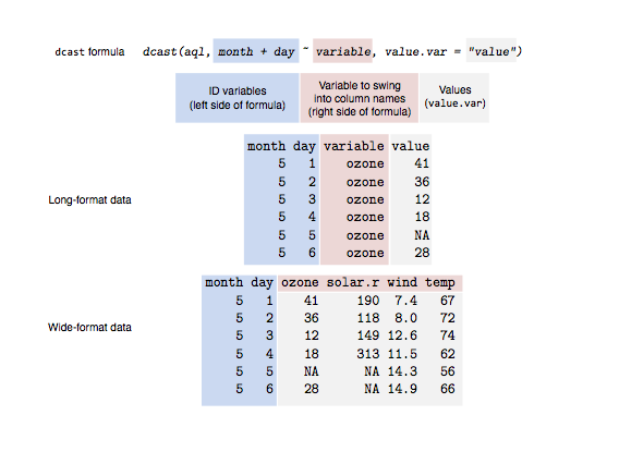
Figure 1: An illustration of the dcast function. The blue shading indicates ID variables that we want to represent individual rows. The red shading represents variable names that we want to swing into column names. The grey shading represents the data values that we want to fill in the cells with.
One confusing “mistake” you might make is casting a dataset in which there is more than one value per data cell. For example, this time we won’t includeday as an ID variable:
dcast(aql, month ~ variable)# month ozone solar.r wind temp# 1 5 31 31 31 31# 2 6 30 30 30 30# 3 7 31 31 31 31# 4 8 31 31 31 31# 5 9 30 30 30 30When you run this in R, you’ll notice the warning message:
# Aggregation function missing: defaulting to lengthAnd if you look at the output, the cells are filled with the number of data rows for each month-climate combination. The numbers we’re seeing are the number of days recorded in each month. When youcast your data and there are multiple values per cell, you also need to telldcast how to aggregate the data. For example, maybe you want to take themean, or the median, or the sum. Let’s try the last example, but this time we’ll take the mean of the climate values. We’ll also pass the optionna.rm = TRUE through the ... argument to remove NA values. (The... let’s you pass on additional arguments to your fun.aggregate function, heremean.)
dcast(aql, month ~ variable, fun.aggregate = mean, na.rm = TRUE)# month ozone solar.r wind temp# 1 5 23.62 181.3 11.623 65.55# 2 6 29.44 190.2 10.267 79.10# 3 7 59.12 216.5 8.942 83.90# 4 8 59.96 171.9 8.794 83.97# 5 9 31.45 167.4 10.180 76.90Unlike melt, there are some other fancy things you can do with dcast that I’m not covering here. It’s worth reading the help file ?dcast. For example, you can compute summaries for rows and columns, subset the columns, and fill in missing cells in one call todcast.
Additional help
Read the package help: help(package = "reshape2")
See the reshape2 website: http://had.co.nz/reshape/
And read the paper on reshape: Wickham, H. (2007). Reshaping data with thereshape package. 21(12):1–20. http://www.jstatsoft.org/v21/i12
(But note that the paper is written for the reshape package not the reshape2 package.)
- An Introduction to reshape2
- An Introduction to Struts
- An introduction to LaTeX2e
- An Introduction To Ajax
- An introduction to SOA
- An introduction to Microcode
- An Introduction to LDAP
- An Introduction To SQLite
- An Introduction to Libaio
- An Introduction to LDAP
- An Introduction to GCC
- An Introduction to OpenCL
- An Introduction to Log4cpp
- An Introduction to ANYDATA
- An Introduction to NFC
- An Introduction to GCC
- An Introduction to ANYDATA
- An introduction to JSON
- SecureCRT端口转发配置
- CentOS 6.4下编译安装MySQL 5.6.14
- 2015机器学习十大问题
- OC总结-block语法
- NDK jni
- An Introduction to reshape2
- 程序员必读书单(非常经典,强烈推荐)
- android使用 webp格式 android使用新格式
- F.NET框架示例(一)
- 微软周四公布了用于Windows 10新浏览器Spartan的渲染引擎细节
- namenode running as process 2405. Stop it first.
- 2013机器学习十大问题
- oracle 10g回收站功能
- 如何分析Android APP 内存大小