从头开始实现一个神经网络

来源：互联网发布：货车软件编辑：程序博客网时间：2024/06/05 00:49

在这篇文章中，我们会从头开始实现一个简单的3层神经网络。我们不会去推导所需的数学公式，但是我会试着给一个直观的解释我们在做什么。我也会指出具体的阅读资源。

在这里我假设您熟悉基本的微积分和机器学习的概念,例如:你知道什么是分类和正规化。理想情况下你也知道一点关于像梯度下降优化技术是如何工作的。但即使你不熟悉任何上面的这篇文章仍有可能是有趣的。

但是为什么从头实现神经网络呢?即使你打算在将来使用像PyBrain的神经网络库,从头开始实现一个神经网络至少一次是一个极其宝贵的锻炼。它可以帮助你获得神经网络如何工作的理解,这是设计有效的模型必不可少的。

需要注意的一件事是,这里的代码示例并不十分有效。他们是容易理解的。在即将发布的我将探索如何使用Theano编写一个有效的神经网络实现。

生成数据集

让我们从生成数据集开始。幸运的是，sciki-learn有一些有用的数据集生成器，所以我们不需要自己编写代码。我们使用make_moons函数

# Generate a dataset and plot itnp.random.seed(0)X, y = sklearn.datasets.make_moons(200, noise=0.20)plt.scatter(X[:,0], X[:,1], s=40, c=y, cmap=plt.cm.Spectral)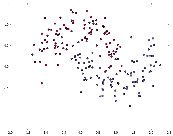

这里写图片描述

我们生成的数据集有两个类,绘制成红色和蓝色的点。你能把蓝点想象为男性患者红点女性患者的,x和y轴是医学测量。

我们的目标是培养一个机器学习分类器预测正确的类(男性女性)的x和y坐标。注意,数据不是线性可分,我们不能画一条直线,两类。这意味着线性分类器、逻辑回归等不能适应数据,除非你hand-engineer非线性特性(如多项式),适合给定的数据集。

事实上,神经网络的主要优势之一。你不需要担心feature engineering。神经网络的隐层将为你学习这些特征。

逻辑回归

为证明这一点让我们训练一个逻辑回归分类器。它的输入是x和y的值，输出是预测类(0或1)。为了方便我们使用scikit-learn来做逻辑回归。

# Train the logistic rgeression classifierclf = sklearn.linear_model.LogisticRegressionCV()clf.fit(X, y)# Plot the decision boundaryplot_decision_boundary(lambda x: clf.predict(x))plt.title("Logistic Regression")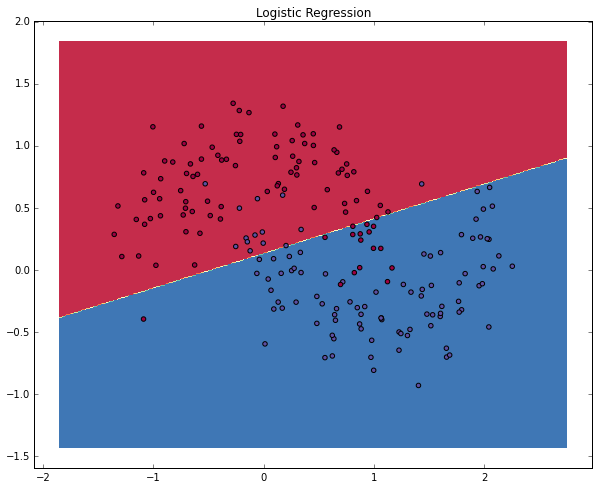

这里写图片描述

图表显示了我们的决策边界学习逻辑回归分类器。它尽可能的用一条直线来分割数据,但这是无法捕捉的“月形”数据。

训练神经网络

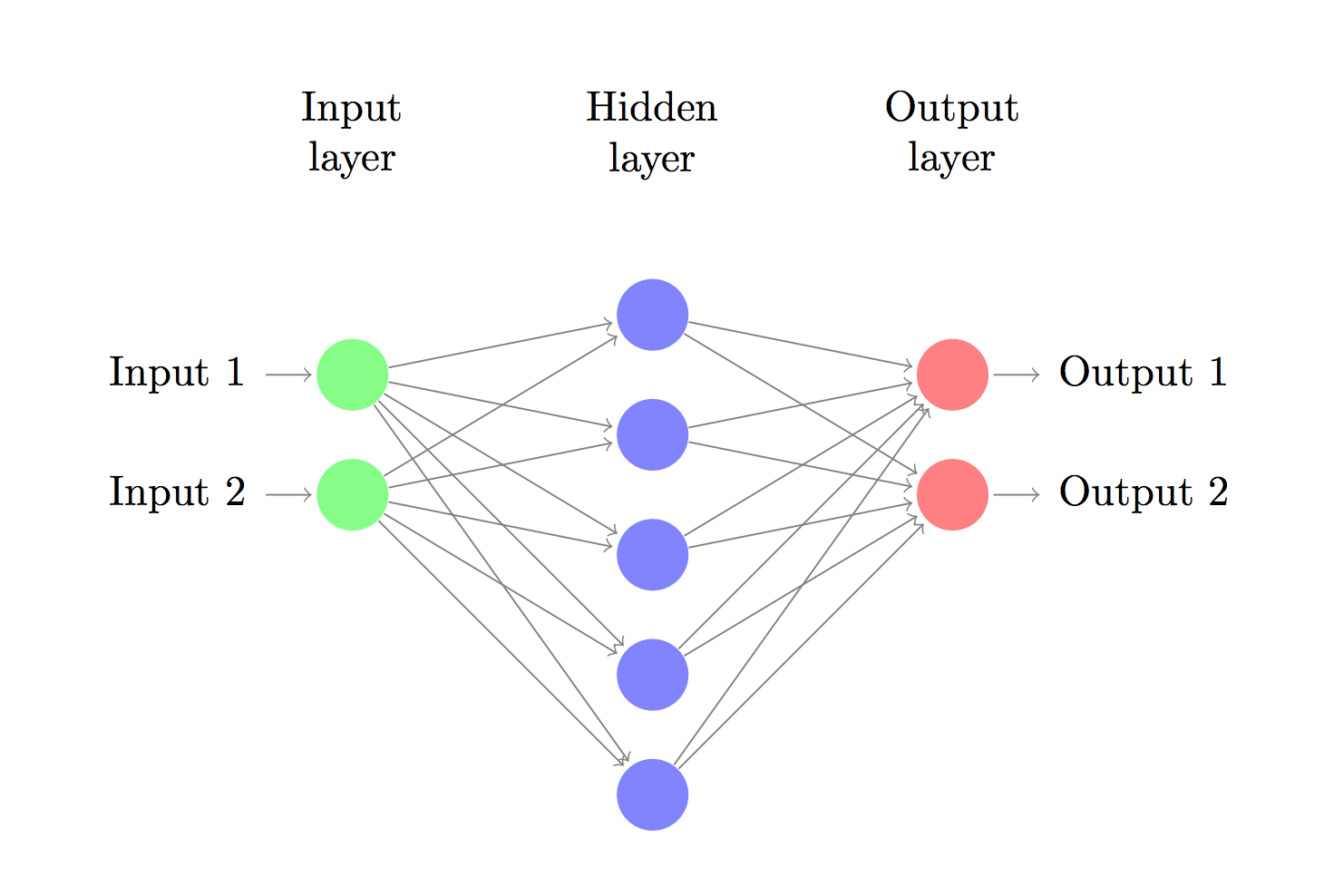
现在让我们用一个输入层、一个隐藏层和一个输出层，来构建一个3 层神经网络。输入层节点的数目是由我们的数据的维数,2。同样,在输出层的节点数量是由类的数量,还2。(因为我们只有2类我们可以只有一个输出节点预测0或1,但是有2更易于扩展网络以后更多的类)。网络的输入将是x和y坐标,其输出将两个可能性,一个用于类0(“女性”),一个用于类1(“男性”)。它看上去是这样的:

这里写图片描述

我们可以选择隐藏层的维数（节点的数目）。隐藏层的节点越多越能拟合复杂的函数。但是，更高的维度是有代价的。首先，更多的计算需要作出预测和学习的网络参数。参数的一个更大的数字也意味着我们变得更容易出现过度拟合我们的数据。

如何选择隐含层的大小？虽然有一些普遍的指导和建议，这总是取决于你的具体问题，更多的是一种艺术，而不是一门科学。我们将尝试不同数量的隐藏层节点，看看它是如何影响我们的输出。

我们还需要为我们的隐藏层选择一个激活函数。激活函数变换输入到其输出。非线性激活函数使我们能够拟合非线性的假设。常见的激活函数有：tanh，sigmoid，或ReLUs。我们将使用tanh，在许多情况下,其表现相当好。这些函数一个很好的属性是它们能够从原函数求导。例如， $t a n h x$ 的导数是 $1 - t a n h^{2} x$ 。这非常有用，因为计算一次 $t a n h x$ 在后面求导能重用.

因为我们希望我们的网络输出激活函数的概率，输出层将是softmax，这是一个简单的方法来原始值转换成概率。如果你熟悉的逻辑函数，你能想到softmax并将其推广到多个类。

我们的神经网络怎样做预测？

我们的网络使用前向传播进行预测，它就是一堆矩阵乘法和我们上面定义的激活函数的应用。如果x是2维的输入，那么我们计算出的约测 $\hat{y}$ (也是2维)，具体如下：

\begin{aligned} z_{1} & = x W_{1} + b_{1} \\ a_{1} & = \tanh (z_{1}) \\ z_{2} & = a_{1} W_{2} + b_{2} \\ a_{2} & = \hat{y} = s o f t m a x (z_{2}) \end{aligned}

$z_{i}$ 是输入层 $i$ , $a_{i}$ 是应用激活函数后的输出层 $i$ . $W_{1}$ , $b_{1}$ , $W_{2}$ , $b_{2}$ 是我们网络的参数，是需要我们通过训练数据学习的。你可以把它们想象成网络层之间的矩阵变换。综观上面的矩阵乘法我们能计算触3个矩阵的维度。如果我们使用500个隐藏节点，那么 $W_{1} \in R^{2 \times 500}$ , $b_{1} \in R^{500}$ , $W_{2} \in R^{500 \times 2}$ , $b_{2} \in R^{2}$ . 现在你应该了解到为什么增加隐藏层的节点我们会有更多的参数了。

参数学习

参数学习意味着找到参数( $W_{1}, b_{1}, W_{2}, b_{2}$ )能够在训练数据上最小化错误。但是，我们怎样定义错误呢？我们称这样的函数是错误损失函数。一般的选择是softmax的交叉熵损失。如果我们有N 个训练样例和C个类别，那么我们预测的 $\hat{y}$ 和期望的 $y$ 的损失是：

\begin{aligned} L (y, \hat{y}) = - \frac{1}{N} \sum_{n \in N} \sum_{i \in C} y_{n, i} \log {\hat{y}}_{n, i} \end{aligned}

公式看起来复杂,但是它确实是我们训练的例子求和，我们预测不正确的类错误的相加。所以,越远 $y$ (正确的标签)和 $\hat{y}$ (我们的预测),我们的损失就越大。

记住,我们的目标是找到最小化我们的损失函数的参数。我们可以使用梯度下降来找到最小。我将实现简化版的梯度下降,也称为批处理梯度下降与一个固定的学习速率。变形的方法如SGD(随机梯度下降)或minibatch梯度下降通常在实践中表现得更好。所以,如果你是认真的你会希望使用其中的一个,和理想情况下你也会降低学习速率。

作为输入,梯度下降需要梯度(向量的导数)的损失函数的参数 $\frac{\partial L}{\partial W_{1}}, \frac{\partial L}{\partial b_{1}}, \frac{\partial L}{\partial W_{2}}, \frac{\partial L}{\partial b_{2}}$ 这些梯度计算我们使用著名的反向传播算法,这是一种有效地从开始到输出计算梯度。我不会详细反向传播是如何工作的,但也有许多优秀的解释(这里和这里)流传于网络。

应用后向传播我们得到如下公式（相信我）：

\begin{aligned} δ_{3} = y - \hat{y} \\ δ_{2} = (1 - \tanh^{2} z_{2}) \circ δ_{3} W_{2}^{T} \\ \frac{\partial L}{\partial W_{2}} = a_{1}^{T} δ_{3} \\ \frac{\partial L}{\partial b_{2}} = δ_{3} \\ \frac{\partial L}{\partial W_{1}} = x^{T} δ 2 \\ \frac{\partial L}{\partial b_{1}} = δ 2 \end{aligned}

实现

现在我们已经为实现做好了准备。我们从定义一些有用的变量和梯度下降的参数开始:

num_examples = len(X) # training set sizenn_input_dim = 2 # input layer dimensionalitynn_output_dim = 2 # output layer dimensionality# Gradient descent parameters (I picked these by hand)epsilon = 0.01 # learning rate for gradient descentreg_lambda = 0.01 # regularization strength

首先，实现我们之前定义的损失函数。我们用它来评估模型：

# Helper function to evaluate the total loss on the datasetdef calculate_loss(model):    W1, b1, W2, b2 = model['W1'], model['b1'], model['W2'], model['b2']    # Forward propagation to calculate our predictions    z1 = X.dot(W1) + b1    a1 = np.tanh(z1)    z2 = a1.dot(W2) + b2    exp_scores = np.exp(z2)    probs = exp_scores / np.sum(exp_scores, axis=1, keepdims=True)    # Calculating the loss    corect_logprobs = -np.log(probs[range(num_examples), y])    data_loss = np.sum(corect_logprobs)    # Add regulatization term to loss (optional)    data_loss += reg_lambda/2 * (np.sum(np.square(W1)) + np.sum(np.square(W2)))    return 1./num_examples * data_loss

我们同时实现一个辅助函数来计算网络的输出。它是之前定义的前向传播并返回类的概率最高。

# Helper function to predict an output (0 or 1)def predict(model, x):    W1, b1, W2, b2 = model['W1'], model['b1'], model['W2'], model['b2']    # Forward propagation    z1 = x.dot(W1) + b1    a1 = np.tanh(z1)    z2 = a1.dot(W2) + b2    exp_scores = np.exp(z2)    probs = exp_scores / np.sum(exp_scores, axis=1, keepdims=True)    return np.argmax(probs, axis=1)

最后,来训练神经网络。它实现了批量使用反向传播梯度下降。

# This function learns parameters for the neural network and returns the model.# - nn_hdim: Number of nodes in the hidden layer# - num_passes: Number of passes through the training data for gradient descent# - print_loss: If True, print the loss every 1000 iterationsdef build_model(nn_hdim, num_passes=20000, print_loss=False):    # Initialize the parameters to random values. We need to learn these.    np.random.seed(0)    W1 = np.random.randn(nn_input_dim, nn_hdim) / np.sqrt(nn_input_dim)    b1 = np.zeros((1, nn_hdim))    W2 = np.random.randn(nn_hdim, nn_output_dim) / np.sqrt(nn_hdim)    b2 = np.zeros((1, nn_output_dim))    # This is what we return at the end    model = {}    # Gradient descent. For each batch...    for i in xrange(0, num_passes):        # Forward propagation        z1 = X.dot(W1) + b1        a1 = np.tanh(z1)        z2 = a1.dot(W2) + b2        exp_scores = np.exp(z2)        probs = exp_scores / np.sum(exp_scores, axis=1, keepdims=True)        # Backpropagation        delta3 = probs        delta3[range(num_examples), y] -= 1        dW2 = (a1.T).dot(delta3)        db2 = np.sum(delta3, axis=0, keepdims=True)        delta2 = delta3.dot(W2.T) * (1 - np.power(a1, 2))        dW1 = np.dot(X.T, delta2)        db1 = np.sum(delta2, axis=0)        # Add regularization terms (b1 and b2 don't have regularization terms)        dW2 += reg_lambda * W2        dW1 += reg_lambda * W1        # Gradient descent parameter update        W1 += -epsilon * dW1        b1 += -epsilon * db1        W2 += -epsilon * dW2        b2 += -epsilon * db2        # Assign new parameters to the model        model = { 'W1': W1, 'b1': b1, 'W2': W2, 'b2': b2}        # Optionally print the loss.        # This is expensive because it uses the whole dataset, so we don't want to do it too often.        if print_loss and i % 1000 == 0:          print "Loss after iteration %i: %f" %(i, calculate_loss(model))    return model

一个3个隐藏层节点的网络

让我们看看如果用3个隐藏层节点的网络来训练会发生什么。

# Build a model with a 3-dimensional hidden layermodel = build_model(3, print_loss=True)# Plot the decision boundaryplot_decision_boundary(lambda x: predict(model, x))plt.title("Decision Boundary for hidden layer size 3")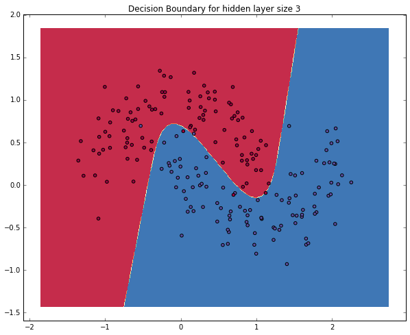

这里写图片描述

耶！这看起来相当不错。我们的神经网络能够找到一个决策边界成功的分类。

不同隐藏层大小

在上面例子中我们国定隐藏层大小为3，让我们看看不过隐藏层大小的结果。

plt.figure(figsize=(16, 32))hidden_layer_dimensions = [1, 2, 3, 4, 5, 20, 50]for i, nn_hdim in enumerate(hidden_layer_dimensions):    plt.subplot(5, 2, i+1)    plt.title('Hidden Layer size %d' % nn_hdim)    model = build_model(nn_hdim)    plot_decision_boundary(lambda x: predict(model, x))plt.show()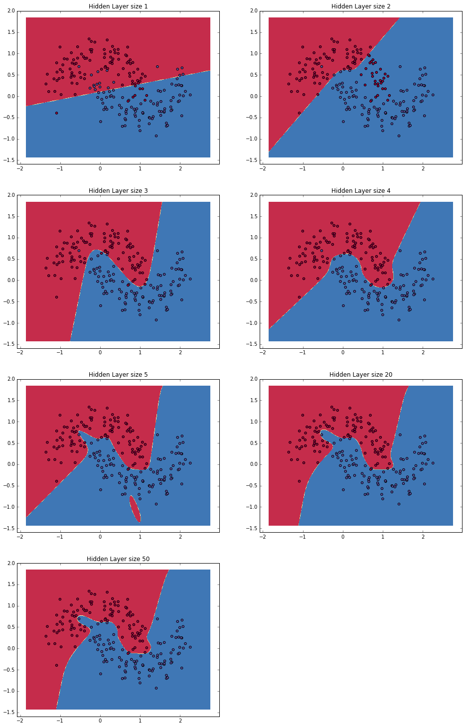

这里写图片描述

我们可以看到,一个隐藏层的低维度很好地捕捉我们的数据的一般趋势。更高的维度容易过度拟合。他们是“记忆”的数据与拟合一般形状。如果我们评估我们的模型在一个单独的测试集(你应该)模型与一个较小的隐层的大小可能会由于更好的泛化表现得更好。我们可以抵消过度拟合通过较强的正则化,但选择隐层的正确的大小是一个更“经济”的解决方案。

练习

这部分不译了。。

Here are some things you can try to become more familiar with the code:

Instead of batch gradient descent, use minibatch gradient descent (more info) to train the network. Minibatch gradient descent typically performs better in practice.
We used a fixed learning rate \epsilon for gradient descent. Implement an annealing schedule for the gradient descent learning rate (more info).
1. We used a \tanh activation function for our hidden layer. Experiment with other activation functions (some are mentioned above). Note that changing the activation function also means changing the backpropagation derivative.
  4.Extend the network from two to three classes. You will need to generate an appropriate dataset for this.
Extend the network to four layers. Experiment with the layer size. Adding another hidden layer means you will need to adjust both the forward propagation as well as the backpropagation code.

All of the code is available as an iPython notebook on Github. Please leave questions or feedback in the comments!

注：代码不能直接跑。这只是主要代码。不过看懂了很容易将加上去了。
原文链接：http://www.wildml.com/2015/09/implementing-a-neural-network-from-scratch/
实验代码：Get the code: To follow along, all the code is also available as an iPython notebook on Github.

0 0