【scikit-learn】scikit-learn的线性回归模型

来源：互联网发布：到期收益率知乎编辑：程序博客网时间：2024/05/22 13:29

【scikit-learn】scikit-learn的线性回归模型

首页
自学中心
软件
PYTHON
【SCIKIT-LEARN】SCIKIT-LEARN的线性回归模型

来自 http://blog.csdn.net/jasonding1354/article/details/46340729

内容概要

如何使用pandas读入数据
如何使用seaborn进行数据的可视化
scikit-learn的线性回归模型和使用方法
线性回归模型的评估测度
特征选择的方法

作为有监督学习，分类问题是预测类别结果，而回归问题是预测一个连续的结果。

1. 使用pandas来读取数据

Pandas是一个用于数据探索、数据处理、数据分析的Python库

In [1]:

import pandas as pd

In [2]:

# read csv file directly from a URL and save the resultsdata = pd.read_csv('http://www-bcf.usc.edu/~gareth/ISL/Advertising.csv', index_col=0)# display the first 5 rowsdata.head()

Out[2]:

TVRadioNewspaperSales1230.137.869.222.1244.539.345.110.4317.245.969.39.34151.541.358.518.55180.810.858.412.9

上面显示的结果类似一个电子表格，这个结构称为Pandas的数据帧(data frame)。

pandas的两个主要数据结构：Series和DataFrame：

Series类似于一维数组，它有一组数据以及一组与之相关的数据标签(即索引)组成。
DataFrame是一个表格型的数据结构，它含有一组有序的列，每列可以是不同的值类型。DataFrame既有行索引也有列索引，它可以被看做由Series组成的字典。

In [3]:

# display the last 5 rowsdata.tail()

Out[3]:

TVRadioNewspaperSales19638.23.713.87.619794.24.98.19.7198177.09.36.412.8199283.642.066.225.5200232.18.68.713.4

In [4]:

# check the shape of the DataFrame(rows, colums)data.shape

Out[4]:

(200, 4)

特征：

TV：对于一个给定市场中单一产品，用于电视上的广告费用（以千为单位）
Radio：在广播媒体上投资的广告费用
Newspaper：用于报纸媒体的广告费用

响应：

Sales：对应产品的销量

在这个案例中，我们通过不同的广告投入，预测产品销量。因为响应变量是一个连续的值，所以这个问题是一个回归问题。数据集一共有200个观测值，每一组观测对应一个市场的情况。

In [5]:

import seaborn as sns%matplotlib inline

In [6]:

# visualize the relationship between the features and the response using scatterplotssns.pairplot(data, x_vars=['TV','Radio','Newspaper'], y_vars='Sales', size=7, aspect=0.8)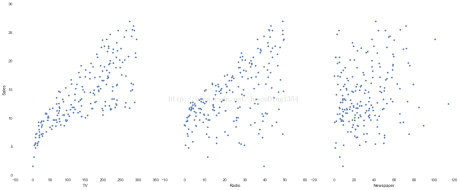

Out[6]:

<seaborn.axisgrid.PairGrid at 0x82dd890>

seaborn的pairplot函数绘制X的每一维度和对应Y的散点图。通过设置size和aspect参数来调节显示的大小和比例。可以从图中看出，TV特征和销量是有比较强的线性关系的，而Radio和Sales线性关系弱一些，Newspaper和Sales线性关系更弱。通过加入一个参数kind=’reg’，seaborn可以添加一条最佳拟合直线和95%的置信带。

In [7]:

sns.pairplot(data, x_vars=['TV','Radio','Newspaper'], y_vars='Sales', size=7, aspect=0.8, kind='reg')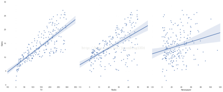

Out[7]:

<seaborn.axisgrid.PairGrid at 0x83b76f0>

2. 线性回归模型

优点：快速；没有调节参数；可轻易解释；可理解

缺点：相比其他复杂一些的模型，其预测准确率不是太高，因为它假设特征和响应之间存在确定的线性关系，这种假设对于非线性的关系，线性回归模型显然不能很好的对这种数据建模。

线性模型表达式： y=β0+β1x1+β2x2+...+βnxn 其中

y是响应
β0是截距
β1是x1的系数，以此类推

在这个案例中： y=β0+β1∗TV+β2∗Radio+...+βn∗Newspaper

（1）使用pandas来构建X和y

scikit-learn要求X是一个特征矩阵，y是一个NumPy向量
pandas构建在NumPy之上
因此，X可以是pandas的DataFrame，y可以是pandas的Series，scikit-learn可以理解这种结构

In [8]:

# create a python list of feature namesfeature_cols = ['TV', 'Radio', 'Newspaper']# use the list to select a subset of the original DataFrameX = data[feature_cols]# equivalent command to do this in one lineX = data[['TV', 'Radio', 'Newspaper']]# print the first 5 rowsX.head()

Out[8]:

TVRadioNewspaper1230.137.869.2244.539.345.1317.245.969.34151.541.358.55180.810.858.4

In [9]:

# check the type and shape of Xprint type(X)print X.shape

<class 'pandas.core.frame.DataFrame'>(200, 3)

In [10]:

# select a Series from the DataFramey = data['Sales']# equivalent command that works if there are no spaces in the column namey = data.Sales# print the first 5 valuesy.head()

Out[10]:

1    22.12    10.43     9.34    18.55    12.9Name: Sales, dtype: float64

In [11]:

print type(y)print y.shape

<class 'pandas.core.series.Series'>(200,)

(2)构造训练集和测试集

In [12]:

from sklearn.cross_validation import train_test_splitX_train, X_test, y_train, y_test = train_test_split(X, y, random_state=1)

In [14]:

# default split is 75% for training and 25% for testingprint X_train.shapeprint y_train.shapeprint X_test.shapeprint y_test.shape

(150, 3)(150,)(50, 3)(50,)

(3)Scikit-learn的线性回归

In [15]:

from sklearn.linear_model import LinearRegressionlinreg = LinearRegression()linreg.fit(X_train, y_train)

Out[15]:

LinearRegression(copy_X=True, fit_intercept=True, n_jobs=1, normalize=False)

In [16]:

print linreg.intercept_print linreg.coef_

2.87696662232[ 0.04656457  0.17915812  0.00345046]

In [17]:

# pair the feature names with the coefficientszip(feature_cols, linreg.coef_)

Out[17]:

[('TV', 0.046564567874150253), ('Radio', 0.17915812245088836), ('Newspaper', 0.0034504647111804482)]

y=2.88+0.0466∗TV+0.179∗Radio+0.00345∗Newspaper

如何解释各个特征对应的系数的意义？

对于给定了Radio和Newspaper的广告投入，如果在TV广告上每多投入1个单位，对应销量将增加0.0466个单位
更明确一点，加入其它两个媒体投入固定，在TV广告上没增加1000美元（因为单位是1000美元），销量将增加46.6（因为单位是1000）

(4)预测

In [18]:

y_pred = linreg.predict(X_test)

3. 回归问题的评价测度

对于分类问题，评价测度是准确率，但这种方法不适用于回归问题。我们使用针对连续数值的评价测度(evaluation metrics)。

下面介绍三种常用的针对回归问题的评价测度

In [21]:

# define true and predicted response valuestrue = [100, 50, 30, 20]pred = [90, 50, 50, 30]

(1)平均绝对误差(Mean Absolute Error, MAE)

1n∑ni=1|yi−yi^|

(2)均方误差(Mean Squared Error, MSE)

1n∑ni=1(yi−yi^)2

(3)均方根误差(Root Mean Squared Error, RMSE)

1n∑ni=1(yi−yi^)2−−−−−−−−−−−−−√

In [24]:

from sklearn import metricsimport numpy as np# calculate MAE by handprint "MAE by hand:",(10 + 0 + 20 + 10)/4.# calculate MAE using scikit-learnprint "MAE:",metrics.mean_absolute_error(true, pred)# calculate MSE by handprint "MSE by hand:",(10**2 + 0**2 + 20**2 + 10**2)/4.# calculate MSE using scikit-learnprint "MSE:",metrics.mean_squared_error(true, pred)# calculate RMSE by handprint "RMSE by hand:",np.sqrt((10**2 + 0**2 + 20**2 + 10**2)/4.)# calculate RMSE using scikit-learnprint "RMSE:",np.sqrt(metrics.mean_squared_error(true, pred))

MAE by hand: 10.0MAE: 10.0MSE by hand: 150.0MSE: 150.0RMSE by hand: 12.2474487139RMSE: 12.2474487139

计算Sales预测的RMSE

In [26]:

print np.sqrt(metrics.mean_squared_error(y_test, y_pred))

1.40465142303

4. 特征选择

在之前展示的数据中，我们看到Newspaper和销量之间的线性关系比较弱，现在我们移除这个特征，看看线性回归预测的结果的RMSE如何？

In [27]:

feature_cols = ['TV', 'Radio']X = data[feature_cols]y = data.SalesX_train, X_test, y_train, y_test = train_test_split(X, y, random_state=1)linreg.fit(X_train, y_train)y_pred = linreg.predict(X_test)print np.sqrt(metrics.mean_squared_error(y_test, y_pred))