OpenCV - Detect skew angle

refer from http://felix.abecassis.me/2011/09/opencv-detect-skew-angle/

OpenCV

Lately I have been interested in the library OpenCV. This library, initially developed by Intel, is dedicated to computer vision applications and is known to be one of the fastest (and maybe the fastest ?) library available for real-time computer vision.

And yet, if you think the library is not fast enough you can install Intel Integrated Performance Primitives (IPP) on your system and benefit from heavily optimized routines. If you have several cores available on your computer, you can also installIntel Threading Building Blocks (TBB). And if it'sstill not fast enough, you can run some operations on your GPU using CUDA !

All these features looked really exciting, so I decided to experiment a little bit with OpenCV in order to test its interface and expressive power. In this article I present a simple and very short project that detects the skew angle of a digitized document. My goal is not to present an error-proof program but rather to show the ease of use of OpenCV.

Skew angle

The detection of the skew angle of a document is a common preprocessing step in document analysis.

The document might have been slightly rotated during its digitization. It is therefore necessary to compute the skew angle and to rotate the text before going further in the processing pipeline (i.e.words/letters segmentation and later OCR).

We will work on 5 different images of the same short (but famous) text.

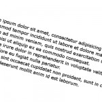
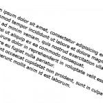
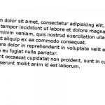
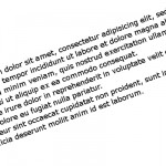
The naming convention for those images is rather simple, the first letter stands for the sign of the angle (p for plus, m for minus) and the following number is the value of the angle.
m8.jpg has therefore been rotated by an angle of -8 degrees.

We assume here that the noise introduced by digitization has been removed by a previous preprocessing stage. We also assume that the text has been isolated: no images, horizontal or vertical separators, etc.

Implementation with OpenCV

First, let's declare a function compute_skew, it takes a path to an image as input and outputs the detected angle to standard output.
First we load the image and stores its size in a variable, very simple.

void compute_skew(const char* filename){   // Load in grayscale.   cv::Mat src = cv::imread(filename, 0);   cv::Size size = src.size();

In image processing, objects are white and the background is black, we have the opposite, we need to invert the colors of our image:

   cv::bitwise_not(src, src);

And here is the result:

In order to compute the skew we must find straight lines in the text. In a text line, we have several letters side by side, lines should therefore be formed by finding long lines of white pixels in the image. Here is an example below:

Of course as characters have an height, we find several lines for each actual line from the text. By fine tuning the parameters used later or by using preprocessing we can decrease the number of lines.

So, how do we find lines in the image ? We use a powerful mathematical tool called theHough transform. I won't dig into mathematical details, but the main idea of the Hough transform is to use a 2D accumulator in order to count how many times a given line has been found in the image, the whole image is scanned and by a voting system the "best" lines are identified.
We used a more efficient variant of the Standard Hough Transform (SHT) called theProbabilistic Hough Transform (PHT). In OpenCV the PHT is implemented under the nameHoughLinesP.

In addition to the standard parameters of the Hough Transform, we have two additional parameters:

• minLineLength – The minimum line length. Line segments shorter than that will be rejected. This is a great tool in order to prune out small residual lines.
• maxLineGap – The maximum allowed gap between points on the same line to link them.
  This could be interesting for a multi-columns text, for example we could choose to not link lines from different text columns.

Back to C++ now, in OpenCV the PHT stores the end points of the line whereas the SHT stores the line in polar coordinates (relative to the origin). We need a vector in order to store all the end points:

    std::vector<cv::Vec4i> lines;

We are ready for the Hough transform now:

    cv::HoughLinesP(src, lines, 1, CV_PI/180, 100, size.width / 2.f, 20);

We use a step size of 1 for ρ and π/180 for θ, the threshold (the minimum number of votes) is 100.
minLineLength is width/2, this is not an unreasonable assumption if the text is well isolated.
maxLineGap is 20, it seems a sound value for a gap.

In the remaining of the code we simply calculate the angle between each line and the horizontal line using theatan2 math function and we compute the mean angle of all the lines.
For debugging purposes we also draw all the lines in a new image called disp_lines and we display this image in a new window.

    cv::Mat disp_lines(size, CV_8UC1, cv::Scalar(0, 0, 0));    double angle = 0.;    unsigned nb_lines = lines.size();    for (unsigned i = 0; i < nb_lines; ++i)    {        cv::line(disp_lines, cv::Point(lines[i][0], lines[i][1]),                 cv::Point(lines[i][2], lines[i][3]), cv::Scalar(255, 0 ,0));        angle += atan2((double)lines[i][3] - lines[i][1],                       (double)lines[i][2] - lines[i][0]);    }    angle /= nb_lines; // mean angle, in radians.     std::cout << "File " << filename << ": " << angle * 180 / CV_PI << std::endl;     cv::imshow(filename, disp_lines);    cv::waitKey(0);    cv::destroyWindow(filename);}

We just need a main function in order to call compute_skew on several images:

const char* files[] = { "m8.jpg", "m20.jpg", "p3.jpg", "p16.jpg", "p24.jpg"}; int main(){unsigned nb_files = sizeof(files) / sizeof(const char*);for (unsigned i = 0; i < nb_files; ++i)compute_skew(files[i]);}

That's all, here are the skew angles we obtain for each image, we have a pretty good accuracy:

refer from http://felix.abecassis.me/2011/10/opencv-bounding-box-skew-angle/

In a previous article I presented how to compute the skew angle of a digitized text document by using the Probabilistic Hough Transform.
In this article we will present another method in order to calculate this angle , this method is less acurate than the previous one but our goal is rather to introduce two new OpenCV techniques: image scan with an iterator and computing the minimum bounding box of a set of points.

Bounding Box

The minimum bounding box of a set of 2D points set is the smallest rectangle (i.e. with smallest area) that contains all the points of the set. Given an image representing a text, like this one:

The points of our 2D set are all the white pixels forming the different letters.
If we can compute the bounding box of this set, it will be possible to compute the skew angle of our document. Given a bounding box of our set, it will also be easy to extract our text from the image and rotate it (probably in a future article).

Preprocessing

Our text is small but we have a large number of points, indeed the resolution of our image is large, we have many pixels per letter. We have several possibilities here: we can downstrongle the image in order to reduce its resolution, we can use mathematical morphology (i.e. erosion), etc. There are certainly other solutions, you will have to choose one depending on what are the previous or next stages in your processing pipeline (e.g. maybe you already have a downstrongled image).

In this article I have chosen to experiment using mathematical morphology for this problem.
We used a 5x3 rectangle shaped structuring element, that is to say we want to keep pixels that lies in a region of white pixels of height 3 and width 5.
Here is the result on the previous image:

Okay, this erosion was really aggressive, we removed most pixels and in fact only some letters "survived" the operation. Calculating the bounding box will be really fast but we may have stripped too much information, it might cause problems on certain images. However as we will see, there are still enough pixels to get decent results.

Implementation

The OpenCV program is similar to the one presented in the previous article.
We declare a compute_skew function that takes as input the path to the image to process, at the beginning of the function we load this image in grayscale, we binarize it and we invert the colors (because objects are represented as white pixels, and the background is represented by black pixels).

void compute_skew(const char* filename){  // Load in grayscale.  cv::Mat img = cv::imread(filename, 0);   // Binarize  cv::threshold(img, img, 225, 255, cv::THRESH_BINARY);   // Invert colors  cv::bitwise_not(img, img);

We can now perform our erosion, we must declare our rectangle-shaped structuring element and call theerode function:

  cv::Mat element = cv::getStructuringElement(cv::MORPH_RECT, cv::Size(5, 3));  cv::erode(img, img, element);

Now we must create our set of points before calling the function computing the bounding box. As this function cannot be called on an image, we must extract all the positions of our white pixels, this is a great opportunity to present how to scan an image using an iterator:

  std::vector<cv::Point> points;  cv::Mat_<uchar>::iterator it = img.begin<uchar>();  cv::Mat_<uchar>::iterator end = img.end<uchar>();  for (; it != end; ++it)    if (*it)      points.push_back(it.pos());

We declare a vector of points in order to store all white pixels. Like when we iterate on a container in C++, we must declare an iterator and also get the iterator representing theend of our container. We use the Mat_ class, note the underscore at the end: it is because it is a templated class: here we must precise the type of the underlying data type. The image has only one channel of size 1 byte, the type is therefore uchar (unsigned char).

We can now use the OpenCV function in order to compute the minimal bounding box, this function is calledminAreaRect, this function need a cv::Mat as input so we must convert our vector of points.

  cv::RotatedRect box = cv::minAreaRect(cv::Mat(points));

That's it, we have our minimal bounding box!
We can now have access to the angle:

  double angle = box.angle;  if (angle < -45.)    angle += 90.;

During testing I notice I only got negative angle and never below -90 degrees. This is because as we have no reference rectangle, there are several ways to compute the rotation angle. In our case, if the angle is less than -45 degrees, the angle was computed using a "vertical" rectangle, we must therefore correct the angle by adding 90 degrees.

Finally, we will display our bounding rectangle on our eroded image and print the angle on standard output:

  cv::Point2f vertices[4];  box.points(vertices);  for(int i = 0; i < 4; ++i)    cv::line(img, vertices[i], vertices[(i + 1) % 4], cv::Scalar(255, 0, 0), 1, CV_AA);   std::cout << "File " << filename << ": " << angle << std::endl;  cv::imshow("Result", img);  cv::waitKey(0);

Note that the line was anti-aliased using CV_AA as the last argument of cv::line.

Results

Using the same 5 images as in the previous article, we obtained the following angles:

The naming convention for those images is simple, the first letter stands for the sign of the angle (p for plus, m for minus) and the following number is the value of the angle.
The results are not as good as in the previous article, especially with a large angle. Indeed with large values, our preprocessing step (the erosion) will be less meaningful because pixels of a single letter are not vertically or horizontally aligned at all.

Note that the bounding box obtained is not the bounding box of our whole text. The erosion removed a lot of information, if we try to match the bounding box on the initial text, we will lose for example the upper part of letters with a larger height that other letters (e.g. f, t, h, d, l...). Compute the bounding box on the unprocessed text (or use a smaller structuring element) if you want the bounding box of the whole text.

refer from http://felix.abecassis.me/2011/10/opencv-rotation-deskewing/

In a previous article I presented how to compute the skew angle of a digitized text document by using the Probabilistic Hough Transform. In thelast article I presented how to compute a bounding box using OpenCV, this method was also used to compute the skew angle but with a reduced accuracy compared to the first method.

Test Set

We will be using the same small test set as before:

The naming convention for those images is simple, the first letter stands for the sign of the angle (p for plus, m for minus) and the following number is the value of the angle.
m8.jpg has therefore been rotated by an angle of -8 degrees.

Bounding Box

In this article I will assume we have computed the skew angle of each image with a good accuracy and we now want to rotate the text by this angle value. We therefore declare a function calleddeskew that takes as parameters the path to the image to process and the skew angle.

void deskew(const char* filename, double angle){  cv::Mat img = cv::imread(filename, 0);   cv::bitwise_not(img, img);   std::vector<cv::Point> points;  cv::Mat_<uchar>::iterator it = img.begin<uchar>();  cv::Mat_<uchar>::iterator end = img.end<uchar>();  for (; it != end; ++it)    if (*it)      points.push_back(it.pos());   cv::RotatedRect box = cv::minAreaRect(cv::Mat(points));

This code is similar to the previous article: we load the image, invert black and white and compute the minimum bounding box. However this time there is no preprocessing stage because we want the bounding box of the whole text.

Rotation

We compute the rotation matrix using the corresponding OpenCV function, we specify the center of the rotation (the center of our bounding box), the rotation angle (the skew angle) and the scale factor (none here).

  cv::Mat rot_mat = cv::getRotationMatrix2D(box.center, angle, 1);

Now that we have the rotation matrix, we can apply the geometric transformation using the functionwarpAffine:

  cv::Mat rotated;  cv::warpAffine(img, rotated, rot_mat, img.size(), cv::INTER_CUBIC);

The 4th argument is the interpolation method. Interpolation is important in this situation, when applying the transformation matrix, some pixels in the destination image might have no predecessor from the source image (think of scaling with a factor 2). Those pixels have no defined value, and the role of interpolation is to fill those gaps by computing a value using the local neighborhood of this pixel.
The quality of the output and the execution speed depends on the method chosen.

The simplest (and fastest) interpolation method is INTER_NEAREST, but it yields awful results:
.

There are four other interpolation methods: INTER_NEAREST, INTER_AREA, INTER_CUBIC and INTER_LANCSOZ4.
For our example those 4 methods yielded visually similar results.
The rotated image using INTER_CUBIC (bicubic interpolation):

Cropping

We should now crop the image in order to remove borders:

  cv::Size box_size = box.size;  if (box.angle < -45.)    std::swap(box_size.width, box_size.height);  cv::Mat cropped;  cv::getRectSubPix(rotated, box_size, box.center, cropped);

As mentioned in the previous article, if the skew angle is positive, the angle of the bounding box is below -45 degrees because the angle is given by taking as a reference a "vertical" rectangle,i.e. with the height greater than the width.
Therefore, if the angle is positive, we swap height and width before calling the cropping function.

Cropping is made using getRectSubPix, you must specify the input image, the size of the output image, the center of the rectangle and finally the output image.
We use the original center because the center of a rotation is invariant through this transformation.
This function works at a sub-pixel accuracy (hence its name): the center of the rectangle can be a floating point value.

The cropped image: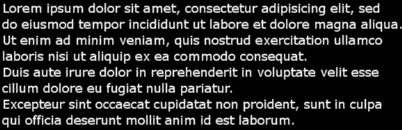

To better understand the problem we have with positive angles, here what you would get without the correction:

We can immediately see that we just need to swap the height and the width of the rectangle.

Display

This is a small demo so let's display the original image, the rotated image and the cropped image:

  cv::imshow("Original", img);  cv::imshow("Rotated", rotated);  cv::imshow("Cropped", cropped);  cv::waitKey(0);}

That's it ! It's really simple to rotate an image with OpenCV !

refer from http://felix.abecassis.me/2011/09/opencv-morphological-skeleton/

Skeleton

In many computer vision applications we often have to deal with huge amounts of data: processing can therefore be slow and requires a lot of memory.
In order to achieve faster processing and a smaller memory footprint, we sometimes use a more compact representation called askeleton.
A skeleton must preserve the structure of the shape but all redundant pixels should be removed.
Here is a skeleton of the letter "B":

In this article we will present how to compute a morphological skeleton with the library OpenCV.
The skeleton obtained is far from perfect but it is a really simple method compared to other existing algorithms.

Pseudocode

As described on Wikipedia, a morphological skeleton can be computed using only the two basic morphological operations: dilate and erode.
In pseudo code, the algorithm works as follow:

img = ...;while (not_empty(img)){    skel = skel | (img & !open(img));    img = erosion(img);}

At each iteration the image is eroded again and the skeleton is refined by computing the union of the current erosion less theopening of this erosion. An opening is simply an erosion followed by a dilation.

Implementation

It's really straightforward, first load the image to process in grayscale and transform it to a binary image using thresholding:

cv::Mat img = cv::imread("O.png", 0);cv::threshold(img, img, 127, 255, cv::THRESH_BINARY);

We now need an image to store the skeleton and also a temporary image in order to store intermediate computations in the loop. The skeleton image is filled with black at the beginning.

cv::Mat skel(img.size(), CV_8UC1, cv::Scalar(0));cv::Mat temp(img.size(), CV_8UC1);

We have to declare the structuring element we will use for our morphological operations, here we use a 3x3 cross-shaped structure element (i.e. we use 4-connexity).

cv::Mat element = cv::getStructuringElement(cv::MORPH_CROSS, cv::Size(3, 3));

And now the core of the algorithm, the main loop. We need a boolean variable in order to check if there is at least one pixel remaining. Operations are done in-place when possible.

bool done;do{  cv::morphologyEx(img, temp, cv::MORPH_OPEN, element);  cv::bitwise_not(temp, temp);  cv::bitwise_and(img, temp, temp);  cv::bitwise_or(skel, temp, skel);  cv::erode(img, img, element);   double max;  cv::minMaxLoc(img, 0, &max);  done = (max == 0);} while (!done);

The use of the minMaxLoc function deserves an explanation. We want to check if there is still at least one pixel in the image, unfortunately I have not found a function for this task in OpenCV, therefore I just check if the maximum value is 0. minMaxLoc stores the minimum value in the second parameter (ignored if NULL pointer) and the maximum in the third parameter. A short-circuit OR function would be nice for this task.

The loop is over, we have our skeleton, let's display it!

cv::imshow("Skeleton", skel);cv::waitKey(0);

Results

On a big "O":

On the word "OpenCV":

Optimization

As discussed with Arthur Kalverboer in the comments below, it is possible to optimize the computation in several ways.

First of all we can notice we perform the open operation and just after we perform anerosion on the same image, but an opening is just an erosion followed by a dilation, so we can perform the erosion and save it to a new imageeroded, and at the end of the loop we copy eroded toimg.

The second optimization concerns the use of cv::minMaxLoc in order to check if an image still has white pixels, computing the norm (cv::norm) of the image is faster.
EDIT2: Abid Rahman told me the function 'cv::countNonZero' is even faster, I didn't know this function existed, thanks!

Finally the last optimization is to replace the and and not operations by a simple set difference operation (cv::subtract). This works because we only manipulate binary images.

Here is the updated code:

cv::threshold(img, img, 127, 255, cv::THRESH_BINARY); cv::Mat skel(img.size(), CV_8UC1, cv::Scalar(0));cv::Mat temp;cv::Mat eroded; cv::Mat element = cv::getStructuringElement(cv::MORPH_CROSS, cv::Size(3, 3)); bool done;do{  cv::erode(img, eroded, element);  cv::dilate(eroded, temp, element); // temp = open(img)  cv::subtract(img, temp, temp);  cv::bitwise_or(skel, temp, skel);  eroded.copyTo(img);   done = (cv::countNonZero(img) == 0);} while (!done);

Also, don't forget to crop your images before processing. The two images I gave as examples are not cropped, cropping them (manually or using OpenCV) also improves execution time.