循环神经网络在Python 、Numpy和Theano中的实现

这篇文章翻译自

实现代码

在这部分，我们将使用Python从头实现一个完整的RNN，并且使用theano进行优化。

语言模型：
我们的目的是使用RNN构建语言模型；
假设我们有包含m个单词的句子，语言模型能够让我们预测这个句子存在的概率；

换句话说，句子存在的概率有每一个单词的概率的乘积得到，单词的概率由它之前的单词决定；
应用领域：
这个模型能够作为一个评分机制，例如，在机器翻译系统中，由一个句子经常生成多个候选答案，能够使用语言模型选择出最可能的答案。直观的，概率最大的句子
更可能语法正确的；
但是处理语言模型问题有一个很酷的副作用；因为我们能够根据前面的单词预测该单词存在的概率，我么能够生成文本；这是一个生成模型，假定存在一个单词序列
我们能够根据预测概率采样出下一个单词。重复这个过程，直到我们能够得到一个完整的句子。
Andrej Karparthy 展示了语言模型能够做些什么？“见我摘录的博客
他的模型把单个字母作为元素进行训练；
注意：上面的公式考虑了每个单词在之前单词存在时的条件概率。在实际中，由于计算复杂度和内存限制的问题，许多模型在表示长期依赖时都比较困难。一般情况下，只关注之前的几个单词。RNN原理上能够捕获长期依赖，但是实际上是相当复杂的。
训练数据与预处理
我们需要文本来训练语言模型。幸运的是，训练语言模型不需要任何的标记。
我下载了15000篇长长的Reddit的评论，下载地址
我的模型生成的文本听起来像真实的评论；但是，像其他的机器学习项目一样，我们需要进行合理的预处理，使数据转化为正确的格式；
标记文本（ TOKENIZE TEXT）：
我们拥有原始文本，但是我们想要基于前面单词进行预测。意味着，必须把评论标记为句子，句子转化为单词；我么能够仅仅通过空格划分评论，但是这样不能够合适的处理标调符号。我们能够使用NLYK的word_tokenize and sent_tokenize methods进行预处理来解决这一难题。
去除罕见的单词（REMOVE INFREQUENT WORDS）
我们文档中的大部分单词将只会出现一两次，把这些不频繁的单词移除是个好的办法。拥有一个巨大的词表将会使我们的模型训练缓慢；因为这些单词没有足够的语境示例，因此不能够学习到正确的使用方式。这就像人学习一样，要想学会合适的使用一个单词，必须在不同的语境中见到它；

在我们的代码中，我们限制单词表的大小为vocabulary_size，仅仅保存最常用的单词。*把所有不在单词表中的单词使用*UNKNOWN_TOKEN 来代替。UNKNOWN_TOKEN将要变成单词表中一部分，我们将要像其他单词一样预测它。
当我们生成了新的文本之后，我们能替换掉它；例如随机的抽取一个不在单词表中的单词进行替换；
在特殊的开始和边界结束（ PREPEND SPECIAL START AND END TOKENS）：
我们想要学习那些单词倾向于开始和结束一个据句子。为了做到这些，我们预先加入 SENTENCE_END 特殊标记和 SENTENCE_START特殊标记到每一个句子；
建立训练数据矩阵（BUILD TRAINING DATA MATRICES）
RNN的输入是向量，而不是字符串。所以首先构建单词与指数之间的映射（index_to_word, and word_to_index. ）。例如，单词”Friendly”在单词表中的序号是2001，一个训练样本x看起来就像[0,179,341,416]，这里0对应 SENTENCE_START，相应的y标签可能就是[179,341,416,1],记住我们的任务就是预测下一个单词。所以y仅仅是x向量移动一位，即最后一个元素是SENTENCE_END token。
这里是我们文本中实际的训练例子：

x:SENTENCE_START what are n't you understanding about this ? ![0, 51, 27, 16, 10, 856, 53, 25, 34, 69]y:what are n't you understanding about this ? ! SENTENCE_END[51, 27, 16, 10, 856, 53, 25, 34, 69, 1]

vocabulary_size = 8000unknown_token = "UNKNOWN_TOKEN"sentence_start_token = "SENTENCE_START"sentence_end_token = "SENTENCE_END"# Read the data and append SENTENCE_START and SENTENCE_END tokensprint "Reading CSV file..."with open('data/reddit-comments-2015-08.csv', 'rb') as f:    reader = csv.reader(f, skipinitialspace=True)    reader.next()    # Split full comments into sentences    sentences = itertools.chain(*[nltk.sent_tokenize(x[0].decode('utf-8').lower()) for x in reader])    # Append SENTENCE_START and SENTENCE_END    sentences = ["%s %s %s" % (sentence_start_token, x, sentence_end_token) for x in sentences]print "Parsed %d sentences." % (len(sentences))# Tokenize the sentences into wordstokenized_sentences = [nltk.word_tokenize(sent) for sent in sentences]# Count the word frequenciesword_freq = nltk.FreqDist(itertools.chain(*tokenized_sentences))print "Found %d unique words tokens." % len(word_freq.items())# Get the most common words and build index_to_word and word_to_index vectorsvocab = word_freq.most_common(vocabulary_size-1)index_to_word = [x[0] for x in vocab]index_to_word.append(unknown_token)word_to_index = dict([(w,i) for i,w in enumerate(index_to_word)])print "Using vocabulary size %d." % vocabulary_sizeprint "The least frequent word in our vocabulary is '%s' and appeared %d times." % (vocab[-1][0], vocab[-1][1])# Replace all words not in our vocabulary with the unknown tokenfor i, sent in enumerate(tokenized_sentences):    tokenized_sentences[i] = [w if w in word_to_index else unknown_token for w in sent]print "\nExample sentence: '%s'" % sentences[0]print "\nExample sentence after Pre-processing: '%s'" % tokenized_sentences[0]# Create the training dataX_train = np.asarray([[word_to_index[w] for w in sent[:-1]] for sent in tokenized_sentences])y_train = np.asarray([[word_to_index[w] for w in sent[1:]] for sent in tokenized_sentences])

构建RNN（BUILDING THE RNN）
下图展示了RNN的总体框架；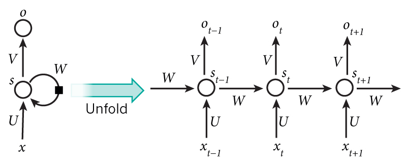

让我们扼要重述RNN的公式

假设选择的词典大小为C=8000,一个隐含层大小为H=100.能够认为隐含层大小为神经网络的存储器，它允许我们学习更加复杂的模型，但导致了额外的计算量。

这是重要的信息，记得U,V，W,是我们想要从数据中学习得到的参数，因此，我们需要总共学习2HC+H^2个参数，这个指标能表明模型的瓶颈，注意到Xt是One-hot向量，它与U相乘进本等同于选择U中的一列，因此不必要执行完整的乘法，而且，最大的向量乘法是VSt，这就是为什么我们想要保持字典的大小越小越好。

初始化（INITIALIZATION）
我们开始创建一个RN你类来初始化我们的参数。把这个类叫做RNNNumpy,因为我们再后来会实现Theano版本。初始化U，V，W参数有一些狡猾，我们不能把它们初始化为零，因为这会导致在所有层中的对称计算。所以一定要随机初始化它们。
因为恰当的初始化会对训练结果产生影响，这在许多研究中已经被证实；实验证明最好的初始化决定于激活函数，一个建议的方法是随机初始化权重在
区间内，n是指从前一层进来的连接数量；这可能听起来过度的复杂，但是用小的随机值初始化它们一般情况会运行的很好；

class RNNNumpy:    def __init__(self, word_dim, hidden_dim=100, bptt_truncate=4):        # Assign instance variables        self.word_dim = word_dim        self.hidden_dim = hidden_dim        self.bptt_truncate = bptt_truncate        # Randomly initialize the network parameters        self.U = np.random.uniform(-np.sqrt(1./word_dim), np.sqrt(1./word_dim), (hidden_dim, word_dim))        self.V = np.random.uniform(-np.sqrt(1./hidden_dim), np.sqrt(1./hidden_dim), (word_dim, hidden_dim))        self.W = np.random.uniform(-np.sqrt(1./hidden_dim), np.sqrt(1./hidden_dim), (hidden_dim, hidden_dim))

上面，word_dim 指单词表的大小，hidden_dim 指隐含层的大小，
bptt_truncate parameter稍后解释；

正向传播（FORWARD PROPAGATION）
接下来，根据前面的公式实现前向传播算法

def forward_propagation(self, x):    # The total number of time steps    T = len(x)    # During forward propagation we save all hidden states in s because need them later.    # We add one additional element for the initial hidden, which we set to 0    s = np.zeros((T + 1, self.hidden_dim))    s[-1] = np.zeros(self.hidden_dim)    # The outputs at each time step. Again, we save them for later.    o = np.zeros((T, self.word_dim))    # For each time step...    for t in np.arange(T):        # Note that we are indxing U by x[t]. This is the same as multiplying U with a one-hot vector.        s[t] = np.tanh(self.U[:,x[t]] + self.W.dot(s[t-1]))        o[t] = softmax(self.V.dot(s[t]))    return [o, s]RNNNumpy.forward_propagation = forward_propagation

我们不仅能够输出计算结果，而且能输出隐含层状态，之后我们将要用他来计算梯度，返回这些值能让我们避免重复计算。每一个输出Ot是一个概率向量，代表词典中的单词，但是有时，例如评价模型的时候，我们只想知道具有最大概率的下一个单词，我们叫它为预测函数

def predict(self, x):    # Perform forward propagation and return index of the highest score    o, s = self.forward_propagation(x)    return np.argmax(o, axis=1)RNNNumpy.predict = predict

让我们尝试一下新的 实践方法，看看示例的输出

def predict(self, x):    # Perform forward propagation and return index of the highest score    o, s = self.forward_propagation(x)    return np.argmax(o, axis=1)RNNNumpy.predict = predict

(45, 8000)[[ 0.00012408  0.0001244   0.00012603 ...,  0.00012515  0.00012488   0.00012508] [ 0.00012536  0.00012582  0.00012436 ...,  0.00012482  0.00012456   0.00012451] [ 0.00012387  0.0001252   0.00012474 ...,  0.00012559  0.00012588   0.00012551] ...,  [ 0.00012414  0.00012455  0.0001252  ...,  0.00012487  0.00012494   0.0001263 ] [ 0.0001252   0.00012393  0.00012509 ...,  0.00012407  0.00012578   0.00012502] [ 0.00012472  0.0001253   0.00012487 ...,  0.00012463  0.00012536   0.00012665]]

对于句子中的每一个单词，我们的模型给出8000个预测，分别表示下一个但是的概率。因为我们随机初始化U，V，W，现在的预测是完全随机的。下面给出所有单词中最高概率预测的单词序号；

predictions = model.predict(X_train[10])print predictions.shapeprint predictions

(45,)[1284 5221 7653 7430 1013 3562 7366 4860 2212 6601 7299 4556 2481 238 2539 21 6548 261 1780 2005 1810 5376 4146 477 7051 4832 4991 897 3485 21 7291 2007 6006 760 4864 2182 6569 2800 2752 6821 4437 7021 7875 6912 3575]

计算损失（CALCULATING THE LOSS）
为了训练我们的网络，我需要一种方法计算它造成的损失，我们称它为损失函数L.
我们的目标是寻找参数U，V，W使之能够在训练数据上损失函数最小化。一个经常用的损失函数是Cross-entropy loss .相关链接
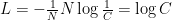
如果我们拥有N个训练样本（文本中的单词个数），和C类（单词表大小），与预测o和正确标签y相关的损失函数定义如下：

这个公式看起来稍微复杂，y与o差距越大，损失函数越大。我们使用calculate_loss 方法进行实现：

def calculate_total_loss(self, x, y):    L = 0    # For each sentence...    for i in np.arange(len(y)):        o, s = self.forward_propagation(x[i])        # We only care about our prediction of the "correct" words        correct_word_predictions = o[np.arange(len(y[i])), y[i]]        # Add to the loss based on how off we were        L += -1 * np.sum(np.log(correct_word_predictions))    return Ldef calculate_loss(self, x, y):    # Divide the total loss by the number of training examples    N = np.sum((len(y_i) for y_i in y))    return self.calculate_total_loss(x,y)/NRNNNumpy.calculate_total_loss = calculate_total_lossRNNNumpy.calculate_loss = calculate_loss

回过头看一下随机预测的损失是多少，它会给我们一个基线，进而确保我们的实现是正确的。在我们的单词表中拥有C个单词，所以每个单词被预测到的概率为1/C，这将会产生损失为

# Limit to 1000 examples to save timeprint "Expected Loss for random predictions: %f" % np.log(vocabulary_size)print "Actual loss: %f" % model.calculate_loss(X_train[:1000], y_train[:1000])

Expected Loss for random predictions: 8.987197Actual loss: 8.987440

使用SGD和反向传播算法训练RNN（TRAINING THE RNN WITH SGD AND BACKPROPAGATION THROUGH TIME ）
记得我们想要得到U，V，W参数，进而最小化训练数据的总体损失。最常用的做法是SGD（随机梯度下降）。SGD背后的思想很简单，我们迭代所有的训练样本，在每次迭代过程中，我们轻微改变参数值使误差减小。改变的方向有损失函数的梯度决定
SGD还需要另一个参数，就是学习率。它决定了每一次迭代一步做出的改变的大小。SGD是最流行的优化函数，不仅仅针对神经网络，而且可用于许多机器学习算法。出现了很多研究通过batching，并行和自适应学习率优化SGD。即使它的思想很简单，以有效的方式实施SGD会变得很复杂。相关链接
如何计算上面提到的梯度呢？在传统的神经网络中，我们通过反向传播算法。在ＲＮＮｓ我们使用这个算法稍微改进的版本，叫做Backpropagation Through Time (BPTT)。因为网络中的参数在所有的时间步骤中共享，每一个输出的梯度不仅仅依赖于当前步的计算，而且还与前面的步骤相关。如果你知道微积分，它实际上用了里面的链式法则，反向传播算法相关文档part1part2
我们把BPTT是为黑盒，它输入训练样本 ，输出梯度；

def bptt(self, x, y):    T = len(y)    # Perform forward propagation    o, s = self.forward_propagation(x)    # We accumulate the gradients in these variables    dLdU = np.zeros(self.U.shape)    dLdV = np.zeros(self.V.shape)    dLdW = np.zeros(self.W.shape)    delta_o = o    delta_o[np.arange(len(y)), y] -= 1.    # For each output backwards...    for t in np.arange(T)[::-1]:        dLdV += np.outer(delta_o[t], s[t].T)        # Initial delta calculation        delta_t = self.V.T.dot(delta_o[t]) * (1 - (s[t] ** 2))        # Backpropagation through time (for at most self.bptt_truncate steps)        for bptt_step in np.arange(max(0, t-self.bptt_truncate), t+1)[::-1]:            # print "Backpropagation step t=%d bptt step=%d " % (t, bptt_step)            dLdW += np.outer(delta_t, s[bptt_step-1])                          dLdU[:,x[bptt_step]] += delta_t            # Update delta for next step            delta_t = self.W.T.dot(delta_t) * (1 - s[bptt_step-1] ** 2)    return [dLdU, dLdV, dLdW]RNNNumpy.bptt = bptt

梯度检测（GRADIENT CHECKING）
无论什么时候你应用反向传播算法，同时实施梯度检测是个好的做法。它是一种验证实践是否正确的方法；梯度检测背后的思想是一个参数的倒数等同于所在点的斜率。我们能够通过轻微改变这个参数+平均改变量进行近似：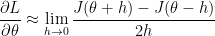

我们然后比较通过梯度下降法计算得到的梯度和通过上式方法估计得到的梯度。若没有太大的差异说明没有问题。这个近似需要计算所有参数总的损失，所以梯度检测代价很大。所以在小的词典的模型中实施很合理；

def gradient_check(self, x, y, h=0.001, error_threshold=0.01):    # Calculate the gradients using backpropagation. We want to checker if these are correct.    bptt_gradients = self.bptt(x, y)    # List of all parameters we want to check.    model_parameters = ['U', 'V', 'W']    # Gradient check for each parameter    for pidx, pname in enumerate(model_parameters):        # Get the actual parameter value from the mode, e.g. model.W        parameter = operator.attrgetter(pname)(self)        print "Performing gradient check for parameter %s with size %d." % (pname, np.prod(parameter.shape))        # Iterate over each element of the parameter matrix, e.g. (0,0), (0,1), ...        it = np.nditer(parameter, flags=['multi_index'], op_flags=['readwrite'])        while not it.finished:            ix = it.multi_index            # Save the original value so we can reset it later            original_value = parameter[ix]            # Estimate the gradient using (f(x+h) - f(x-h))/(2*h)            parameter[ix] = original_value + h            gradplus = self.calculate_total_loss([x],[y])            parameter[ix] = original_value - h            gradminus = self.calculate_total_loss([x],[y])            estimated_gradient = (gradplus - gradminus)/(2*h)            # Reset parameter to original value            parameter[ix] = original_value            # The gradient for this parameter calculated using backpropagation            backprop_gradient = bptt_gradients[pidx][ix]            # calculate The relative error: (|x - y|/(|x| + |y|))            relative_error = np.abs(backprop_gradient - estimated_gradient)/(np.abs(backprop_gradient) + np.abs(estimated_gradient))            # If the error is to large fail the gradient check            if relative_error > error_threshold:                print "Gradient Check ERROR: parameter=%s ix=%s" % (pname, ix)                print "+h Loss: %f" % gradplus                print "-h Loss: %f" % gradminus                print "Estimated_gradient: %f" % estimated_gradient                print "Backpropagation gradient: %f" % backprop_gradient                print "Relative Error: %f" % relative_error                return            it.iternext()        print "Gradient check for parameter %s passed." % (pname)RNNNumpy.gradient_check = gradient_check# To avoid performing millions of expensive calculations we use a smaller vocabulary size for checking.grad_check_vocab_size = 100np.random.seed(10)model = RNNNumpy(grad_check_vocab_size, 10, bptt_truncate=1000)model.gradient_check([0,1,2,3], [1,2,3,4])

SGD实施（SGD IMPLEMENTATION）
既然现在我们能够计算我们参数的梯度，我们能够实施SGD。可分为两步：
1.方法sdg_step计算梯度，实施一批更新。
2.外层循环迭代训练集，自适应学习率。

# Performs one step of SGD.def numpy_sdg_step(self, x, y, learning_rate):    # Calculate the gradients    dLdU, dLdV, dLdW = self.bptt(x, y)    # Change parameters according to gradients and learning rate    self.U -= learning_rate * dLdU    self.V -= learning_rate * dLdV    self.W -= learning_rate * dLdWRNNNumpy.sgd_step = numpy_sdg_step

# Outer SGD Loop# - model: The RNN model instance# - X_train: The training data set# - y_train: The training data labels# - learning_rate: Initial learning rate for SGD# - nepoch: Number of times to iterate through the complete dataset# - evaluate_loss_after: Evaluate the loss after this many epochsdef train_with_sgd(model, X_train, y_train, learning_rate=0.005, nepoch=100, evaluate_loss_after=5):    # We keep track of the losses so we can plot them later    losses = []    num_examples_seen = 0    for epoch in range(nepoch):        # Optionally evaluate the loss        if (epoch % evaluate_loss_after == 0):            loss = model.calculate_loss(X_train, y_train)            losses.append((num_examples_seen, loss))            time = datetime.now().strftime('%Y-%m-%d %H:%M:%S')            print "%s: Loss after num_examples_seen=%d epoch=%d: %f" % (time, num_examples_seen, epoch, loss)            # Adjust the learning rate if loss increases            if (len(losses) > 1 and losses[-1][1] > losses[-2][1]):                learning_rate = learning_rate * 0.5                 print "Setting learning rate to %f" % learning_rate            sys.stdout.flush()        # For each training example...        for i in range(len(y_train)):            # One SGD step            model.sgd_step(X_train[i], y_train[i], learning_rate)            num_examples_seen += 1

完成！让我们试这感觉一下训练这个网络花费的时间；

np.random.seed(10)model = RNNNumpy(vocabulary_size)%timeit model.sgd_step(X_train[10], y_train[10], 0.005)

不好的消息是，我在的电脑上SGD的第一步花费了将近350微秒，我们的训练数据中拥有大概80000个样本，所以训练中的一次迭代将要花费几个小时，多次迭代将要花费好多天。即使是这样，相比于公司和研究机构，我们处理的仍然是小数据集。
幸运的是有很多的方法用来加速代码的运行。我们能够坚持模型不变而把代码运行更快，或者改变我们的模型是指拥有更少的计算量。例如，通过使用分层softmax或者加入投影层来避免大的矩阵乘法。相关文档http://www.fit.vutbr.cz/research/groups/speech/publi/2011/mikolov_icassp2011_5528.pdf“>part1 https://arxiv.org/pdf/1301.3781.pdf“>part2
但是想要保持模型加简单：能够通过使用GPU是我们的应用运行速度更快。
在此之前，我们试着在小的数据集上运行SGD，检测损失值实际中是否变小：

np.random.seed(10)# Train on a small subset of the data to see what happensmodel = RNNNumpy(vocabulary_size)losses = train_with_sgd(model, X_train[:100], y_train[:100], nepoch=10, evaluate_loss_after=1)

2015-09-30 10:08:19: Loss after num_examples_seen=0 epoch=0: 8.9874252015-09-30 10:08:35: Loss after num_examples_seen=100 epoch=1: 8.9762702015-09-30 10:08:50: Loss after num_examples_seen=200 epoch=2: 8.9602122015-09-30 10:09:06: Loss after num_examples_seen=300 epoch=3: 8.9304302015-09-30 10:09:22: Loss after num_examples_seen=400 epoch=4: 8.8622642015-09-30 10:09:38: Loss after num_examples_seen=500 epoch=5: 6.9135702015-09-30 10:09:53: Loss after num_examples_seen=600 epoch=6: 6.3024932015-09-30 10:10:07: Loss after num_examples_seen=700 epoch=7: 6.0149952015-09-30 10:10:24: Loss after num_examples_seen=800 epoch=8: 5.8338772015-09-30 10:10:39: Loss after num_examples_seen=900 epoch=9: 5.710718

很好，好像我们的实现至少做了一下有用的事情，减少了损失值

运用Theano和GPU训练网络（TRAINING OUR NETWORK WITH THEANO AND THE GPU）

关于theano的教程thenao教程
定义一个RNNTheano class 它用在Theao中的相对应的计算替换numpy计算。代码下载地址

np.random.seed(10)model = RNNTheano(vocabulary_size)%timeit model.sgd_step(X_train[10], y_train[10], 0.005)

这时，SGP这一步在没有安装GPU的mac上花费了70ms，在装有GPU的 g2.2xlarge Amazon EC2 instance上花费了23ms
为了避免花费数天时间来训练模型，我已经预训练了一个Theao模型，它包含一个50维的隐含层，单词表大小为8000。训练花费了20小时进行了50次迭代。损失仍在减小，训练更长时间将会得到一个更好的模型。你能够在data/trained-model-theano.npz 中寻找到模型参数。使用load_model_parameters_theano 函数进行加载它们：、

from utils import load_model_parameters_theano, save_model_parameters_theanomodel = RNNTheano(vocabulary_size, hidden_dim=50)# losses = train_with_sgd(model, X_train, y_train, nepoch=50)# save_model_parameters_theano('./data/trained-model-theano.npz', model)load_model_parameters_theano('./data/trained-model-theano.npz', model)

既然有了自己的模型，就可以利用它生成新的文本，让我们实现一个生成新句子的更有效的方法；

def generate_sentence(model):    # We start the sentence with the start token    new_sentence = [word_to_index[sentence_start_token]]    # Repeat until we get an end token    while not new_sentence[-1] == word_to_index[sentence_end_token]:        next_word_probs = model.forward_propagation(new_sentence)        sampled_word = word_to_index[unknown_token]        # We don't want to sample unknown words        while sampled_word == word_to_index[unknown_token]:            samples = np.random.multinomial(1, next_word_probs[-1])            sampled_word = np.argmax(samples)        new_sentence.append(sampled_word)    sentence_str = [index_to_word[x] for x in new_sentence[1:-1]]    return sentence_strnum_sentences = 10senten_min_length = 7for i in range(num_sentences):    sent = []    # We want long sentences, not sentences with one or two words    while len(sent) < senten_min_length:        sent = generate_sentence(model)    print " ".join(sent)

生成的句子：
Anyway, to the city scene you’re an idiot teenager.
What ? ! ! ! ! ignore!
Screw fitness, you’re saying: https
Thanks for the advice to keep my thoughts around girls.
Yep, please disappear with the terrible generation.
观察生成的句子，有一些有趣的事情值得注意，这个模型能够很好的学习语法，它能个把标点符号放在合适的位置。
然而，大多数生成的句子无法理解或有文法错误。可能由于训练不够充分。但这很可能不是主要的原因，vanillaRNN不能够生成有意义的文本，因为它不能学习单词之间的依赖关系。这也是RNN最初不流行的原因。它在理论上很完美，但是实际上不可行，
幸运的是，训练RNNs的困难现在更容易理解了，下一课程将要讲述BPTT算法，说明什么叫做梯度损失。这回趋势我们学习更加复杂的神经网络，例如LATM，它在处理NLP任务中表现出色。所有这个教程学习到的东西同样适用于LSTM和其他的一些RNN模型
程序下载地址