【图像处理】图像显著性论文—Frequency-tuned Salient Region Detection
来源:互联网 发布:手机号正则表达式js 编辑:程序博客网 时间:2024/06/05 18:07
《Robust Frequency-tuned Salient Region Detection》
https://pdfs.semanticscholar.org/f26f/84a870f8a7b8fcaea404ba0b10fc1e331a8a.pdf
《Frequency-tuned Salient Region Detection》
https://infoscience.epfl.ch/record/135217/files/1708.pdf
设计模式六大原则(1):单一职责原则
图像显著性论文(六)—Saliency Filters Contrast Based Filtering for Salient Region Detection
图像显著性论文(五)——Global Contrast based Salient Region Detection
图像显著性论文(四)—Context-Aware Saliency Detection
图像显著性论文(三)—Frequency-tuned Salient Region Detection
图像显著性论文(二)—Saliency Detection: A Spectral Residual Approach
图像显著性论文(一)—A Model of saliency Based Visual Attention for Rapid Scene Analysis
版权声明:本文为博主原创文章,未经博主允许不得转载。
目录(?)[+]
国庆十一长假回来,是得收收心学习学习了,不过国庆也没去那里玩,因为这人实在是不敢恭维啊,连站的地方都没有了,中国这人口就是吓死人。最近有那么一点点时间,就赶紧把自己感兴趣的学一学,要不然过一阵子老板又给项目就没时间学了,那么就接着我们的图像显著性学习之旅吧!这一篇不想介绍得太详细了,因为这一篇说到的显著性计算实在是太简单了,两条公式就搞定了,但为什么引用率这么高呢,因为它把图像显著性提升到应用层面上来了,使人们更多的关注整个显著性区域而不是以前显著性论文所讲的,只有一些注视点。
1、其他显著性方法介绍
现在的显著性方法可以大致分为三类,分别是 biologically based, purely computational, or a combination,基于biologically的有Itti的 A model of saliency-based visual attention for rapid scene analysis也就是第一篇介绍的论文,基于purely computational的有X. Hou and L. Zhang 的Saliency detection: A spectral residual approach也即是第二篇介绍的论文,基于combination的有J. Harel, C. Koch, and P. Perona的Graph-based visualsaliency也即是biological和computational的结合。在频率域分别对5种显著性方法进行讨论,5种方法分别是IT,MZ,GB,SR,AC。由于这五种方法在尺度空间对图像频率都有一定的损失,所以最后产生的模糊的显著图,如下图所示。


表2说明了每种方法最后产生的显著图的频率范围,图像大小,复杂度,从上图和表中可以看出IG方法即本文方法保存的图像信息比较全,并且输出的是全分辨率图像。

2、本文方法介绍
对于一个显著性区域而不是注视点,应该满足以下5点要求:

设Wlc为低频阈值,Whc为高频阈值,为了满足第一点,强调最大的显著性目标,所以Wlc必须非常小,这也满足第二点要求,强调整体显著性区域;为了很好的定义显著性目标的边界,所以需要保留高频部分,于是Whc需要高一点,满足第三个要求,但是又要忽略掉一些噪声,即第四个要求,所以也不能太高。从以上的分析可以得出,我们最后需要一个较宽的频率范围[Wlc,Whc]。
这里使用多个高斯差分的结合作为我们的带通滤波器。下图为高斯差分公式。

当我们设定两个高斯方差成一定比例时,如1:1.6,则高斯差分的联合可由下面公式给出

当我们取的比例为1.6时,则每做一次高斯差分,就是一个边缘检测器,那么将所有的高斯差分结合起来,就相当于把所有的边缘检测器从不同的尺度空间中结合起来,这也就说明了为什么显著区域会全部被覆盖而只是得到一些边缘或者点。(简单的说就是每做一次高斯差分就保留一定范围的频率,把所有的高斯差分结合起来就是把所有的频率搜集起来,就达到我们的要求了),所以参数的选择很重要。文章中介绍确定σ1、σ2我们便可以得到一个频带,但是用一个具有实际带宽的频带去处理图像往往得不到我们想要的效果,这里,取σ1为无穷大,当σ1为无穷大时,对图像的滤波就是计算整幅图像的平均值,而σ2取一个小的高斯核,可以滤去一些噪声。最后得到方程为:

先对图像进行高斯滤波,得到滤波后的图像,取其像素点的Lab值Iwhc(x,y),然后计算图像在LAB空间的均值Iμ,最后求欧氏距离,得到显著图。工作流程如下:

3、图像分割
以上就是图像显著图提取的介绍,非常简单,但是优点还是很明显的,特别是作者把它应用在图像分割上,效果很好。
本次分割主要有两个内容:①使用meanshift对图像进行分割;②介绍一种依赖于显著性图的自适应分割方法
分割步骤:
1、用meanshift方法将原图片分割成K大块;
2、计算每一块对应的显著图的平均值Sk;
3、计算整幅显著图的平均值Sμ;
4、计算自适应阈值Ta=2*Sμ;
5、当Sk>Ta时,则认为该区域为显著性图,保留;
工作过程为:

本文参考资料
1、Frequency-tuned Salient Region Detection原文
2、http://ivrgwww.epfl.ch/supplementary_material/RK_CVPR09/(本方法主页和图片、代码下载)
3、四种简单的图像显著性区域特征提取方法-----> AC/HC/LC/FT
4、PPT介绍
自己实现了一下,将代码改为OpenCV代码,运行环境是vs2010+OpenCV2.4.8,运行结果如下,未加图像分割代码。

================================================================
Frequency-tuned Salient Region Detection
Radhakrishna Achanta, Sheila Hemami, Francisco Estrada, and Sabine Susstrunk
Abstract
Detection of visually salient image regions is useful for applications like object segmentation, adaptive compression, and object recognition. In this paper, we introduce a method for salient region detection that outputs full resolution saliency maps with well-defined boundaries of salient objects. These boundaries are preserved by retaining substantially more frequency content from the original image than other existing techniques. Our method exploits features of color and luminance, is simple to implement, and is computationally efficient. We compare our algorithm to five state-of-the-art salient region detection methods with a frequency domain analysis, ground truth, and a salient object segmentation application. Our method outperforms the five algorithms both on the ground truth evaluation and on the segmentation task by achieving both higher precision and better recall.
Reference and PDF
R. Achanta, S. Hemami, F. Estrada and S. Süsstrunk, Frequency-tuned Salient Region Detection, IEEE International Conference on Computer Vision and Pattern Recognition (CVPR 2009), pp. 1597 - 1604, 2009.
[detailed record] [bibtex]
Introduction
Salient regions and objects stand-out with respect to their neighborhood. The goal of our work was to compute the degree of standing out or saliency of each pixel with respect to its neighbourhood in terms of its color and lightness properties. Most saliency detection methods take a similar center-versus-surround approach. One of the key decisions to make is the size of the neighborhood used for computing saliency. In our case we use the entire image as the neighborhood. This allows us to exploit more spatial frequencies than state-of-the-art methods (please refer to the paper for details) resulting in uniformly highlighted salient regions with well-defined borders. 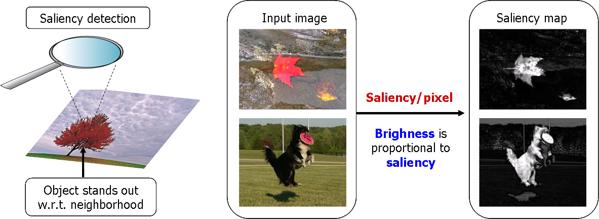
Saliency Detection Algorithm
In simple words, our method find the Euclidean distance between the Lab pixel vector in a Gaussian filtered image with the average Lab vector for the input image. This is illustrated in the figure below. The URL's provided right below the image provide a comparison of our method with state-of-the-art methods. 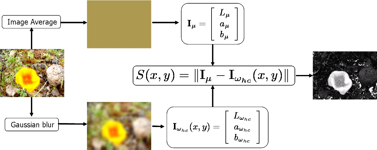
Salient Region Segmentation Algorithm
The salient region segmentation algorithm illustrated below is a modified version of the one presented in [5]. There are two differences with respect to the previous algorith: instead of k-means segmentation mean-shift segmentation is used, and the threshold for choosing salient regions is adaptive (to the average saliency of the input image). 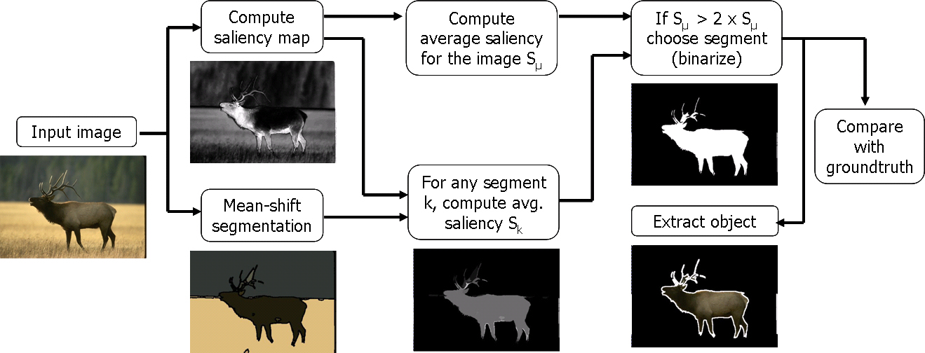
Results
Saliency maps from 5 state-of-the art methods compared to ours (similar to Fig. 3 in the paper).Speed comparison of saliency detection methods.
Salient region segmentation results using our saliency maps (more results similar to Fig. 6 in the paper).
Downloads
1. Ground truth Used for Comparison
We derive a ground truth database of 1000 image from the one presented in [6]. The ground truth in [6] is user-drawn rectangles around salient regions. This is inaccurate and clubs multiple objects into one. We manually-segment the salient object(s) within the user-drawn rectangle to obtain binary masks as shown below. Such masks are both accurate and allows us to deal with multiple salient objects distinctly. The ground truth database can be downloaded from the URL provided below the illustration. 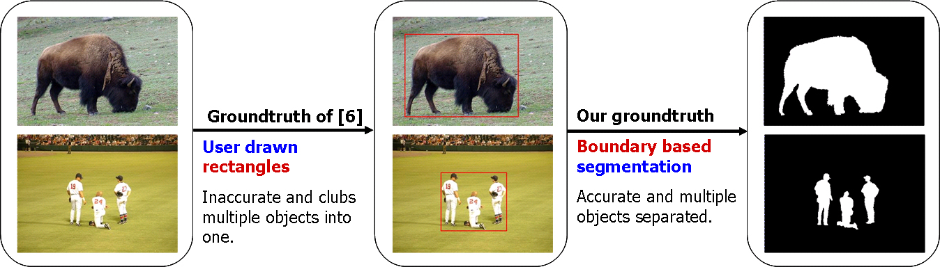
Ground truth of 1000 images
Read me
2. Third party saliency maps for comparison
Saliency maps for the 1000 images using methods IT, MZ, GB, SR, AC, and IG (the maps are normalized to have values between 0 and 255)3. Windows executable
Windows executable for saliency map generation.Usage notes and disclaimer
4. Source Code (C++, MS Visual Studio 2008 workspace)
Salient Region DetectionSalient Region Detection and Segmentation
5. Source Code (MATLAB)
Saliency_CVPR2009.mReferences
[1] L. Itti, C. Koch, and E. Niebur. A model of saliency-based visual attention for rapid scene analysis. PAMI 1998.
[2] Y.-F. Ma and H.-J. Zhang. Contrast-based image attention analysis by using fuzzy growing. ACM MM 2003.
[3] J. Harel, C. Koch, and P. Perona. Graph-based visual saliency. NIPS 2007.
[4] X. Hou and L. Zhang. Saliency detection: A spectral residual approach. CVPR 2007.
[5] R. Achanta, F. Estrada, P. Wils, and S. Süsstrunk. Salient region detection and segmentation. ICVS 2008.
[6] Z. Wang and B. Li. A two-stage approach to saliency detection in images. ICASSP 2008.
Acknowledgements
This work is in part supported by the National Competence Center in Research on Mobile Information and Communication Systems (NCCR-MICS), a center supported by the Swiss National Science Foundation under grant number 5005-67322, the European Commission under contract FP6-027026 (K-Space), and the PHAROS project funded by the European Commission under the 6th Framework Programme (IST Contract No. 045035).
Erratum
The precision-recall curve presented in the paper (Figure 5) was for the first 500 images. The figure for 1000 images that should have been in the paper is shown below. The color conversion function was reimplemented. It shows our method to be doing better than in the figure in the paper. One can reproduce this curve using the C++ code provided for download on this page. Also, Tf values indicated on in Figure 5 can be misleading. Please note that the precision and recall values for a given threshold do not necessarily fall on a vertical line for each of the curves. So in the figure below we are doing away with Tf. 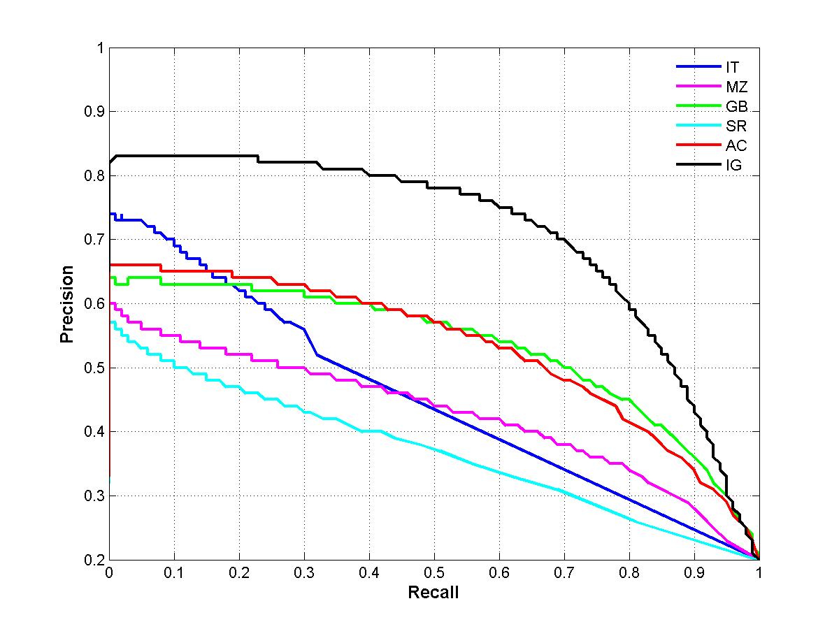
- 【图像处理】图像显著性论文—Frequency-tuned Salient Region Detection
- 图像显著性论文(三)—Frequency-tuned Salient Region Detection
- 阅读图像显著性检测论文二:Frequency-tuned Salient Region Detection
- Frequency-tuned salient Region Detection
- 图像显著性论文(五)——Global Contrast based Salient Region Detection
- 图像显著性论文(六)—Saliency Filters Contrast Based Filtering for Salient Region Detection
- 阅读图像显著性检测论文四:Saliency Filters Contrast Based Filtering for Salient Region Detection
- Frequency-tuned Salient Region Detection:一种快速显著物体检测算法
- 阅读图像显著性检测论文五:2011年版本的Global Contrast Based Salient Region Detection
- 阅读图像显著性检测论文六:2015年版本的Global Contrast Based Salient Region Detection
- Frequency-tuned Salient Region Detection 算法学习总结
- 显著检测论文解析1——Global contrast based salient region detection(程明明 IEEE TPAMI)
- 显著性检测(Salient Detection)
- 图像显著性论文(二)—Saliency Detection: A Spectral Residual Approach
- 图像显著性论文(四)—Context-Aware Saliency Detection
- 图像显著区域检测代码及其效果图 saliency region detection
- 阅读图像显著性检测论文三:Saliency Detection A Spectral Residual Approach
- 图像显著性论文(1-3)
- Qt精美控件
- C++拷贝构造函数详解
- k均值聚类算法
- 字符串匹配及替换 C实现
- 字符编码相关概念理解
- 【图像处理】图像显著性论文—Frequency-tuned Salient Region Detection
- 点击其他程序中的按钮
- 玩转Xcode之修改系统生成的注释模板
- java中的反射机制对属性和方法的操作
- 网络入门视频教程
- Spark集群三种部署模式的区别
- 收集博客
- epoll机制:epoll_create、epoll_ctl、epoll_wait、close
- commons-email实现发送邮件及遇到的问题