利用Caffe做回归(regression)

转自：http://www.cnblogs.com/frombeijingwithlove/p/5314042.html

Caffe应该是目前深度学习领域应用最广泛的几大框架之一了，尤其是视觉领域。绝大多数用Caffe的人，应该用的都是基于分类的网络，但有的时候也许会有基于回归的视觉应用的需要，查了一下Caffe官网，还真没有很现成的例子。这篇举个简单的小例子说明一下如何用Caffe和卷积神经网络（CNN: Convolutional Neural Networks）做基于回归的应用。

原理

最经典的CNN结构一般都是几个卷积层，后面接全连接（FC: Fully Connected）层，最后接一个Softmax层输出预测的分类概率。如果把图像的矩阵也看成是一个向量的话，CNN中无论是卷积还是FC，就是不断地把一个向量变换成另一个向量（事实上对于单个的filter/feature channel，Caffe里最基础的卷积实现就是向量和矩阵的乘法：Convolution in Caffe: a memo），最后输出就是一个把制定分类的类目数作为维度的概率向量。因为神经网络的风格算是黑盒子学习，所以很直接的想法就是把最后输出的向量的值直接拿来做回归，最后优化的目标函数不再是cross entropy等，而是直接基于实数值的误差。

EuclideanLossLayer

Caffe内置的EuclideanLossLayer就是用来解决上面提到的实值回归的一个办法。EuclideanLossLayer计算如下的误差：

12N∑i=1N∥x1i−x2i∥2212N∑i=1N∥xi1−xi2∥22

所以很简单，把标注的值和网络计算出来的值放到EuclideanLossLayer比较差异就可以了。

给图像混乱程度打分的简单例子

用一个给图像混乱程度打分的简单例子来说明如何使用Caffe和EuclideanLossLayer进行回归。

生成基于Ising模型的数据

这里采用统计物理里非常经典的Ising模型的模拟来生成图片，Ising模型可能是统计物理里被人研究最多的模型之一，不过这篇不是讲物理，就略过细节，总之基于这个模型的模拟可以生成如下的图片：

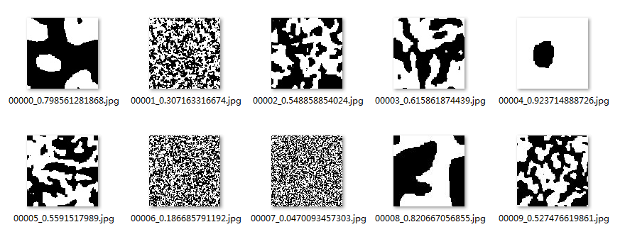
图片中第一个字段是编号，第二个字段对应的分数可以大致认为是图片的有序程度，范围0~1，而这个例子要做的事情就是用一个CNN学习图片的有序程度并预测。

生成图片的Python脚本源于Monte Carlo Simulation of the Ising Model using Python，基于Metropolis算法对Ising模型的模拟，做了一些并行和随机生成图片的修改，在每次模拟的时候随机取一个时间（1e3到1e7之间）点输出到图片，代码如下：

import osimport sysimport datetimefrom multiprocessing import Processimport numpy as npfrom matplotlib import pyplotLATTICE_SIZE = 100SAMPLE_SIZE = 12000STEP_ORDER_RANGE = [3, 7]SAMPLE_FOLDER = 'samples'#----------------------------------------------------------------------##   Check periodic boundary conditions#----------------------------------------------------------------------#def bc(i):    if i+1 > LATTICE_SIZE-1:        return 0    if i-1 < 0:        return LATTICE_SIZE - 1    else:        return i#----------------------------------------------------------------------##   Calculate internal energy#----------------------------------------------------------------------#def energy(system, N, M):    return -1 * system[N,M] * (system[bc(N-1), M] \                               + system[bc(N+1), M] \                               + system[N, bc(M-1)] \                               + system[N, bc(M+1)])#----------------------------------------------------------------------##   Build the system#----------------------------------------------------------------------#def build_system():    system = np.random.random_integers(0, 1, (LATTICE_SIZE, LATTICE_SIZE))    system[system==0] = - 1    return system#----------------------------------------------------------------------##   The Main monte carlo loop#----------------------------------------------------------------------#def main(T, index):    score = np.random.random()    order = score*(STEP_ORDER_RANGE[1]-STEP_ORDER_RANGE[0]) + STEP_ORDER_RANGE[0]    stop = np.int(np.round(np.power(10.0, order)))    print('Running sample: {}, stop @ {}'.format(index, stop))    sys.stdout.flush()    system = build_system()    for step in range(stop):        M = np.random.randint(0, LATTICE_SIZE)        N = np.random.randint(0, LATTICE_SIZE)        E = -2. * energy(system, N, M)        if E <= 0.:            system[N,M] *= -1        elif np.exp(-1./T*E) > np.random.rand():            system[N,M] *= -1        #if step % 100000 == 0:        #    print('.'),        #    sys.stdout.flush()    filename = '{}/'.format(SAMPLE_FOLDER) + '{:0>5d}'.format(index) + '_{}.jpg'.format(score)    pyplot.imsave(filename, system, cmap='gray')    print('Saved to {}!\n'.format(filename))    sys.stdout.flush()#----------------------------------------------------------------------##   Run the menu for the monte carlo simulation#----------------------------------------------------------------------#def run_main(index, length):    np.random.seed(datetime.datetime.now().microsecond)    for i in xrange(index, index+length):        main(0.1, i)def run():    cmd = 'mkdir -p {}'.format(SAMPLE_FOLDER)    os.system(cmd)    n_processes = 8    length = int(SAMPLE_SIZE/n_processes)    processes = [Process(target=run_main, args=(x, length)) for x in np.arange(n_processes)*length]    for p in processes:        p.start()        for p in processes:        p.join()if __name__ == '__main__':    run()

在这个例子中一共随机生成了12000张100x100的灰度图片，命名的规则是[编号]_[有序程度].jpg。至于有序程度为什么用0~1之间的随机数而不是模拟的时间步数，是因为虽说理论上三层神经网络就能逼近任意函数，不过具体到实际训练中还是应该对数据进行预处理，尤其是当目标函数是L2 norm的形式时，如果能保持数据分布均匀，模型的收敛性和可靠性都会提高，范围0到1之间是为了方便最后一层Sigmoid输出对比，同时也方便估算模型误差。还有一点需要注意是，因为图片本身就是模特卡罗模拟产生的，所以即使是同样的有序度的图片，其实看上去不管是主观还是客观的有序程度都是有差别的。

还要提一句的是。。我用Ising的模拟作为例子只是因为很喜欢这个模型，其实用随机相位的反傅里叶变换然后二值化就能得到几乎没什么差别的图像，有序程度就是截止频率，并且更快更简单。

生成训练/验证/测试集

把Ising模拟生成的12000张图片划分为三部分：1w作为训练数据；1k作为验证集；剩下1k作为测试集。下面的Python代码用来生成这样的训练集和验证集的列表：

import osimport numpyfilename2score = lambda x: x[:x.rfind('.')].split('_')[-1]img_files = sorted(os.listdir('samples'))with open('train.txt', 'w') as train_txt:    for f in img_files[:10000]:        score = filename2score(f)        line = 'samples/{} {}\n'.format(f, score)        train_txt.write(line)with open('val.txt', 'w') as val_txt:    for f in img_files[10000:11000]:        score = filename2score(f)        line = 'samples/{} {}\n'.format(f, score)        val_txt.write(line)with open('test.txt', 'w') as test_txt:    for f in img_files[11000:]:        line = 'samples/{}\n'.format(f)        test_txt.write(line)

生成HDF5文件

lmdb虽然又快又省空间，可是Caffe默认的生成lmdb的工具(convert_imageset)不支持浮点类型的数据，虽然caffe.proto里Datum的定义似乎是支持的，不过相应的代码改动还是比较麻烦。相比起来HDF又慢又占空间，但简单好用，如果不是海量数据，还是个不错的选择，这里用HDF来存储用于回归训练和验证的数据，下面是一个生成HDF文件和供Caffe读取文件列表的脚本：

import sysimport numpyfrom matplotlib import pyplotimport h5pyIMAGE_SIZE = (100, 100)MEAN_VALUE = 128filename = sys.argv[1]setname, ext = filename.split('.')with open(filename, 'r') as f:    lines = f.readlines()numpy.random.shuffle(lines)sample_size = len(lines)imgs = numpy.zeros((sample_size, 1,) + IMAGE_SIZE, dtype=numpy.float32)scores = numpy.zeros(sample_size, dtype=numpy.float32)h5_filename = '{}.h5'.format(setname)with h5py.File(h5_filename, 'w') as h:    for i, line in enumerate(lines):        image_name, score = line[:-1].split()        img = pyplot.imread(image_name)[:, :, 0].astype(numpy.float32)        img = img.reshape((1, )+img.shape)        img -= MEAN_VALUE        imgs[i] = img        scores[i] = float(score)        if (i+1) % 1000 == 0:            print('processed {} images!'.format(i+1))    h.create_dataset('data', data=imgs)    h.create_dataset('score', data=scores)with open('{}_h5.txt'.format(setname), 'w') as f:    f.write(h5_filename)

需要注意的是Caffe中HDF的DataLayer不支持transform，所以数据存储前就提前进行了减去均值的步骤。保存为gen_hdf.py，依次运行命令生成训练集和验证集：

python gen_hdf.py train.txt
python gen_hdf.py val.txt

训练

用一个简单的小网络训练这个基于回归的模型：

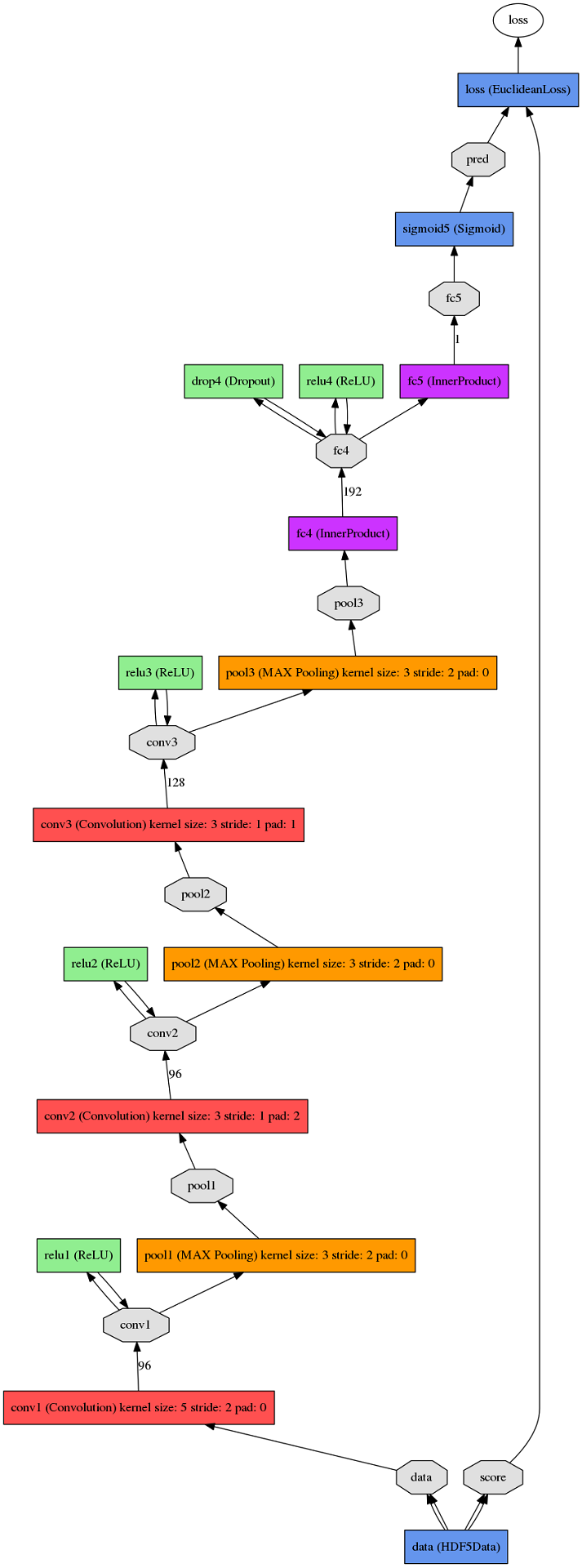
网络结构的train_val.prototxt如下：

name: "RegressionExample"layer {  name: "data"  type: "HDF5Data"  top: "data"  top: "score"  include {    phase: TRAIN  }  hdf5_data_param {    source: "train_h5.txt"    batch_size: 64  }}layer {  name: "data"  type: "HDF5Data"  top: "data"  top: "score"  include {    phase: TEST  }  hdf5_data_param {    source: "val_h5.txt"    batch_size: 64  }}layer {  name: "conv1"  type: "Convolution"  bottom: "data"  top: "conv1"  param {    lr_mult: 1    decay_mult: 1  }  param {    lr_mult: 1    decay_mult: 0  }  convolution_param {    num_output: 96    kernel_size: 5    stride: 2    weight_filler {      type: "gaussian"      std: 0.01    }    bias_filler {      type: "constant"      value: 0    }  }}layer {  name: "relu1"  type: "ReLU"  bottom: "conv1"  top: "conv1"}layer {  name: "pool1"  type: "Pooling"  bottom: "conv1"  top: "pool1"  pooling_param {    pool: MAX    kernel_size: 3    stride: 2  }}layer {  name: "conv2"  type: "Convolution"  bottom: "pool1"  top: "conv2"  param {    lr_mult: 1    decay_mult: 1  }  param {    lr_mult: 1    decay_mult: 0  }  convolution_param {    num_output: 96    pad: 2    kernel_size: 3    weight_filler {      type: "gaussian"      std: 0.01    }    bias_filler {      type: "constant"      value: 0    }  }}layer {  name: "relu2"  type: "ReLU"  bottom: "conv2"  top: "conv2"}layer {  name: "pool2"  type: "Pooling"  bottom: "conv2"  top: "pool2"  pooling_param {    pool: MAX    kernel_size: 3    stride: 2  }}layer {  name: "conv3"  type: "Convolution"  bottom: "pool2"  top: "conv3"  param {    lr_mult: 1    decay_mult: 1  }  param {    lr_mult: 1    decay_mult: 0  }  convolution_param {    num_output: 128    pad: 1    kernel_size: 3    weight_filler {      type: "gaussian"      std: 0.01    }    bias_filler {      type: "constant"      value: 0    }  }}layer {  name: "relu3"  type: "ReLU"  bottom: "conv3"  top: "conv3"}layer {  name: "pool3"  type: "Pooling"  bottom: "conv3"  top: "pool3"  pooling_param {    pool: MAX    kernel_size: 3    stride: 2  }}layer {  name: "fc4"  type: "InnerProduct"  bottom: "pool3"  top: "fc4"  param {    lr_mult: 1    decay_mult: 1  }  param {    lr_mult: 1    decay_mult: 0  }  inner_product_param {    num_output: 192    weight_filler {      type: "gaussian"      std: 0.005    }    bias_filler {      type: "constant"      value: 0    }  }}layer {  name: "relu4"  type: "ReLU"  bottom: "fc4"  top: "fc4"}layer {  name: "drop4"  type: "Dropout"  bottom: "fc4"  top: "fc4"  dropout_param {    dropout_ratio: 0.35  }}layer {  name: "fc5"  type: "InnerProduct"  bottom: "fc4"  top: "fc5"  param {    lr_mult: 1    decay_mult: 1  }  param {    lr_mult: 1    decay_mult: 0  }  inner_product_param {    num_output: 1    weight_filler {      type: "gaussian"      std: 0.005    }    bias_filler {      type: "constant"      value: 0    }  }}layer {  name: "sigmoid5"  type: "Sigmoid"  bottom: "fc5"  top: "pred"}layer {  name: "loss"  type: "EuclideanLoss"  bottom: "pred"  bottom: "score"  top: "loss"}

其中回归部分由EuclideanLossLayer中比较最后一层的输出和train.txt/val.txt中的分数差并作为目标函数实现。需要提一句的是基于实数值的回归问题，对于方差这种目标函数，SGD的性能和稳定性一般来说都不是很好，Caffe文档里也有提到过这点。不过具体到Caffe中，能用就行。。solver.prototxt如下：

net: "./train_val.prototxt"test_iter: 2000test_interval: 500base_lr: 0.01lr_policy: "step"gamma: 0.1stepsize: 50000display: 50max_iter: 10000momentum: 0.85weight_decay: 0.0005snapshot: 1000snapshot_prefix: "./example_ising"solver_mode: GPUtype: "Nesterov"

然后训练：

/path/to/caffe/build/tools/caffe train -solver solver.prototxt

测试

随便训了10000个iteration，反正是收敛了

把train_val.prototxt的两个data layer替换成input_shape，然后去掉最后一层EuclideanLoss就可以了，input_shape定义如下：

input: "data"input_shape {  dim: 1  dim: 1  dim: 100  dim: 100}

改好后另存为deploy.prototxt，然后把训好的模型拿来在测试集上做测试，pycaffe提供了非常方便的接口，用下面脚本输出一个文件列表里所有文件的预测结果：

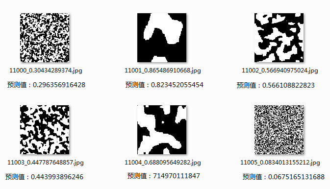
import sysimport numpysys.path.append('/opt/caffe/python')import caffeWEIGHTS_FILE = 'example_ising_iter_10000.caffemodel'DEPLOY_FILE = 'deploy.prototxt'IMAGE_SIZE = (100, 100)MEAN_VALUE = 128caffe.set_mode_cpu()net = caffe.Net(DEPLOY_FILE, WEIGHTS_FILE, caffe.TEST)net.blobs['data'].reshape(1, 1, *IMAGE_SIZE)transformer = caffe.io.Transformer({'data': net.blobs['data'].data.shape})transformer.set_transpose('data', (2,0,1))transformer.set_mean('data', numpy.array([MEAN_VALUE]))transformer.set_raw_scale('data', 255)image_list = sys.argv[1]with open(image_list, 'r') as f:    for line in f.readlines():        filename = line[:-1]        image = caffe.io.load_image(filename, False)        transformed_image = transformer.preprocess('data', image)        net.blobs['data'].data[...] = transformed_image        output = net.forward()        score = output['pred'][0][0]        print('The predicted score for {} is {}'.format(filename, score))

对test.txt执行后，前20个文件的结果：

The predicted score for samples/11000_0.30434289374.jpg is 0.296356916428
The predicted score for samples/11001_0.865486910668.jpg is 0.823452055454
The predicted score for samples/11002_0.566940975024.jpg is 0.566108822823
The predicted score for samples/11003_0.447787648857.jpg is 0.443993896246
The predicted score for samples/11004_0.688095649282.jpg is 0.714970111847
The predicted score for samples/11005_0.0834013155212.jpg is 0.0675165131688
The predicted score for samples/11006_0.421206628337.jpg is 0.419887691736
The predicted score for samples/11007_0.579389741639.jpg is 0.58779758215
The predicted score for samples/11008_0.428772434501.jpg is 0.422569811344
The predicted score for samples/11009_0.188864264594.jpg is 0.18296033144
The predicted score for samples/11010_0.328103100948.jpg is 0.325099766254
The predicted score for samples/11011_0.131306426901.jpg is 0.119059860706
The predicted score for samples/11012_0.627027363247.jpg is 0.622474730015
The predicted score for samples/11013_0.0857273267817.jpg is 0.0735778361559
The predicted score for samples/11014_0.870007364446.jpg is 0.883266746998
The predicted score for samples/11015_0.0515036691772.jpg is 0.0575885437429
The predicted score for samples/11016_0.799989222638.jpg is 0.750781834126
The predicted score for samples/11017_0.22049410733.jpg is 0.208014890552
The predicted score for samples/11018_0.882973794598.jpg is 0.891137182713
The predicted score for samples/11019_0.686353385772.jpg is 0.671325206757
The predicted score for samples/11020_0.385639405472.jpg is 0.385150641203

看上去还不错，挑几张看看：

再输出第一层的卷积核看看：

可以看到第一层的卷积核成功学到了高频和低频的成分，这也是这个例子中判断有序程度的关键，其实就是高频的图像就混乱，低频的就相对有序一些。Ising的自旋图虽然都是二值的，不过学出来的模型也可以随便拿一些别的图片试试：

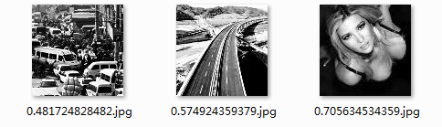
嗯。。定性看还是差不多的。