Analysis of 【Dropout】

原文：https://pgaleone.eu/deep-learning/regularization/2017/01/10/anaysis-of-dropout/

这篇分析dropout的比较好，记录一下。译文在http://www.wtoutiao.com/p/649MGEJ.html

Overfitting is a problem in Deep Neural Networks (DNN): the model learns to classify only the training set, adapting itself to the training examples instead of learning decision boundaries capable of classifying generic instances. Many solutions to the overfitting problem have been presented during these years; one of them have overwhelmed the others due to its simplicity and its empirical good results: Dropout.

Dropout

Visual representation of Dropout, right from the paper. On the left there's the network before applying Dropout, on the right the same network with Dropout applied.
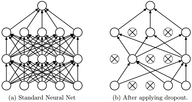
The network on the left it's the same network used at test time, once the parameters have been learned.

---

The idea behind Dropout is to train an ensemble of DNNs and average the results of the whole ensemble instead of train a single DNN.

The DNNs are built dropping out neurons with pp probability, therefore keeping the others on with probability q=1−pq=1−p. When a neuron is dropped out, its output is set to zero, no matter what the input or the associated learned parameter is.

The dropped neurons do not contribute to the training phase in both the forward and backward phases of back-propagation: for this reason every time a single neuron is dropped out it’s like the training phase is done on a new network.

Quoting the authors:

In a standard neural network, the derivative received by each parameter tells it how it should change so the final loss function is reduced, given what all other units are doing. Therefore, units may change in a way that they fix up the mistakes of the other units. This may lead to complex co-adaptations. This in turn leads to overfitting because these co-adaptations do not generalize to unseen data. We hypothesize that for each hidden unit, Dropout prevents co-adaptation by making the presence of other hidden units unreliable. Therefore, a hidden unit cannot rely on other specific units to correct its mistakes.

In short: Dropout works well in practice because it prevents the co-adaption of neurons during the training phase.

Now that we got an intuitive idea behind Dropout, let’s analyze it in depth.

How Dropout works

As said before, Dropout turns off neurons with probability pp and therefore let the others turned on with probability q=1−pq=1−p.

Every single neuron has the same probability of being turned off. This means that:

Given

• h(x)=xW+bh(x)=xW+b a linear projection of a didi-dimensional input xx in a dhdh-dimensional output space.
• a(h)a(h) an activation function

it’s possible to model the application of Dropout, in the training phase only, to the given projection as a modified activation function:

f(h)=D⊙a(h)f(h)=D⊙a(h)

Where D=(X1,⋯,Xdh)D=(X1,⋯,Xdh) is a dhdh-dimensional vector of Bernoulli variables XiXi.

A Bernoulli random variable has the following probability mass distribution:

f(k;p)={p1−pifk=1ifk=0f(k;p)={pifk=11−pifk=0

Where kk are the possible outcomes.

It’s evident that this random variable perfectly models the Dropout application on a single neuron. In fact, the neuron is turned off with probability p=P(k=1)p=P(k=1) and kept on otherwise.

It can be useful to see the application of Dropout on a generic i-th neuron:

Oi=Xia(∑k=1diwkxk+b)={a(∑dik=1wkxk+b)0ifXi=1ifXi=0Oi=Xia(∑k=1diwkxk+b)={a(∑k=1diwkxk+b)ifXi=10ifXi=0

where P(Xi=0)=pP(Xi=0)=p.

Since during train phase a neuron is kept on with probability qq, during the testing phase we have to emulate the behavior of the ensemble of networks used in the training phase.

To do this, the authors suggest scaling the activation function by a factor of qq during the test phase in order to use the expected output produced in the training phase as the single output required in the test phase. Thus:

Train phase: Oi=Xia(∑dik=1wkxk+b)Oi=Xia(∑k=1diwkxk+b)

Test phase: Oi=qa(∑dik=1wkxk+b)Oi=qa(∑k=1diwkxk+b)

Inverted Dropout

A slightly different approach is to use Inverted Dropout. This approach consists in the scaling of the activations during the training phase, leaving the test phase untouched.

The scale factor is the inverse of the keep probability: 11−p=1q11−p=1q, thus:

Train phase: Oi=1qXia(∑dik=1wkxk+b)Oi=1qXia(∑k=1diwkxk+b)

Test phase: Oi=a(∑dik=1wkxk+b)Oi=a(∑k=1diwkxk+b)

Inverted Dropout is how Dropout is implemented in practice in the various deep learning frameworks because it helps to define the model once and just change a parameter (the keep/drop probability) to run train and test on the same model.

Direct Dropout, instead, force you to modify the network during the test phase because if you don’t multiply by qq the output the neuron will produce values that are higher respect to the one expected by the successive neurons (thus the following neurons can saturate or explode): that’s why Inverted Dropout is the more common implementation.

Dropout of a set of neurons

It can be easily noticed that a layer hh with nn neurons, in a single train step, can be seen as an ensemble of nn Bernoulli experiments, each one with a probability of success equals to pp.

Thus, the output of the layer hh have a number of dropped neurons equals to:

Y=∑i=1dhXiY=∑i=1dhXi

Since every neuron is now modeled as a Bernoulli random variable and all these random variables are independent and identically distributed, the total number of dropped neuron is a random variable too, called Binomial:

Y∼Bi(dh,p)Y∼Bi(dh,p)

Where the probability of getting exactly kk success in nn trials is given by the probability mass distribution:

f(k;n,p)=(nk)pk(1−p)n−kf(k;n,p)=(nk)pk(1−p)n−k

This formula can be easily explained:

• pk(1−p)n−kpk(1−p)n−k is the probability of getting a single sequence of kk successes on nntrials and therefore n−kn−k failures.
• (nk)(nk) is the binomial coefficient used to calculate the number of possible sequence of success.

We can now use this distribution to analyze the probability of dropping a specified number of neurons.

When using Dropout, we define a fixed Dropout probability pp for a chosen layer and we expect that a proportional number of neurons are dropped from it.

For example, if the layer we apply Dropout to has n=1024n=1024 neurons and p=0.5p=0.5, we expect that 512 get dropped. Let’s verify this statement:

YP(Y=512)=∑i=11024Xi∼Bi(1024,0.5)=(1024512)0.5512(1−0.5)1024−512≈0.025Y=∑i=11024Xi∼Bi(1024,0.5)P(Y=512)=(1024512)0.5512(1−0.5)1024−512≈0.025

Thus, the probability of dropping out exactly np=512np=512 neurons is of only 0.0250.025!

A python 3 script can help us to visualize how neurons are dropped for different values of pp and a fixed value of nn. The code is commented.

The binomial distribution is very peaked around

npnp

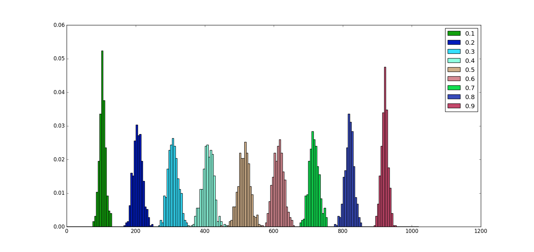
As we can see from the image above no matter what the pp value is, the number of neurons dropped on average is proportional to npnp, in fact:

E[Bi(n,p)]=npE[Bi(n,p)]=np

Moreover, we can notice that the distribution of values is almost symmetric around p=0.5p=0.5 and the probability of dropping npnp neurons increase as the distance from p=0.5p=0.5 increase.

The scaling factor has been added by the authors to compensate the activation values, because they expect that during the training phase only a percentage of 1−p1−pneurons have been kept. During the testing phase, instead, the 100%100% of neurons are kept on, thus the value should be scaled down accordingly.

Dropout & other regularizers

Dropout is often used with L2 normalization and other parameter constraint techniques (such as Max Norm 1), this is not a case. Normalizations help to keep model parameters value low, in this way a parameter can’t grow too much.

In brief, the L2 normalization (for example) is an additional term to the loss, where λ∈[0,1]λ∈[0,1] is an hyper-parameter called regularization strength, F(W;x)F(W;x) is the model and EE is the error function between the real yy and the predicted y^y^ value.

L(y,y^)=E(y,F(W;x))+λ2W2L(y,y^)=E(y,F(W;x))+λ2W2

It’s easy to understand that this additional term, when doing back-propagation via gradient descent, reduces the update amount. If ηη is the learning rate, the update amount of the parameter w∈Ww∈W is

w←w−η(∂F(W;x)∂w+λw)w←w−η(∂F(W;x)∂w+λw)

Dropout alone, instead, does not have any way to prevent parameter values from becoming too large during this update phase. Moreover, the inverted implementation leads the update steps to become bigger, as showed below.

Inverted Dropout and other regularizers

Since Dropout does not prevent parameters from growing and overwhelming each other, applying L2 regularization (or any other regularization technique that constraints the parameter values) can help.

Making explicit the scaling factor, the previous equation becomes:

w←w−η(1q∂F(W;x)∂w+λw)w←w−η(1q∂F(W;x)∂w+λw)

It can be easily seen that when using Inverted Dropout, the learning rate is scaled by a factor of qq. Since qq has values in ]0,1]]0,1] the ratio between ηη and qq can vary between:

r(q)=ηq∈[η=limq→1r(q),+∞=limq→0r(q)]r(q)=ηq∈[η=limq→1r(q),+∞=limq→0r(q)]

For this reason, from now on we’ll call qq boosting factor because it boosts the learning rate. Moreover, we’ll call r(q)r(q) the effective learning rate.

The effective learning rate, thus, is higher respect to the learning rate chosen: for this reason normalizations that constrain the parameter values can help to simplify the learning rate selection process.

Summary

1. Dropout exists in two versions: direct (not commonly implemented) and inverted
2. Dropout on a single neuron can be modeled using a Bernoulli random variable
3. Dropout on a set of neurons can be modeled using a Binomial random variable
4. Even if the probability of dropping exactly npnp neurons is low, npnp neurons are dropped on average on a layer of nn neurons.
5. Inverted Dropout boost the learning rate
6. Inverted Dropout should be using together with other normalization techniques that constrain the parameter values in order to simplify the learning rate selection procedure
7. Dropout helps to prevent overfitting in deep neural networks.

1. Max Norm impose a constraint to the parameters size. Chosen a value for the hyper-parameter cc it impose the constraint |w|≤c|w|≤c. ↩

Share this post!