深度学习基础之：理解卷积学习笔记 （一）：卷积

 目的：

为更深入的研究和探索卷积神经网络，以便实现结构和理论上的创新。 为了做到这一点，我们需要非常深刻地理解卷积。

1.colah's blog: Understanding Convolutions

Lessons from a Dropped Ball

Imagine we drop a ball from some height onto the ground, where it only has one dimension of motion. How likely is it that a ball will go a distance cc if you drop it and then drop it again from above the point at which it landed?

Let’s break this down. After the first drop, it will land aa units away from the starting point with probability f(a)fa, where ff is the probability distribution.

Now after this first drop, we pick the ball up and drop it from another height above the point where it first landed. The probability of the ball rolling bb units away from the new starting point is g(b)gb, where gg may be a different probability distribution if it’s dropped from a different height.

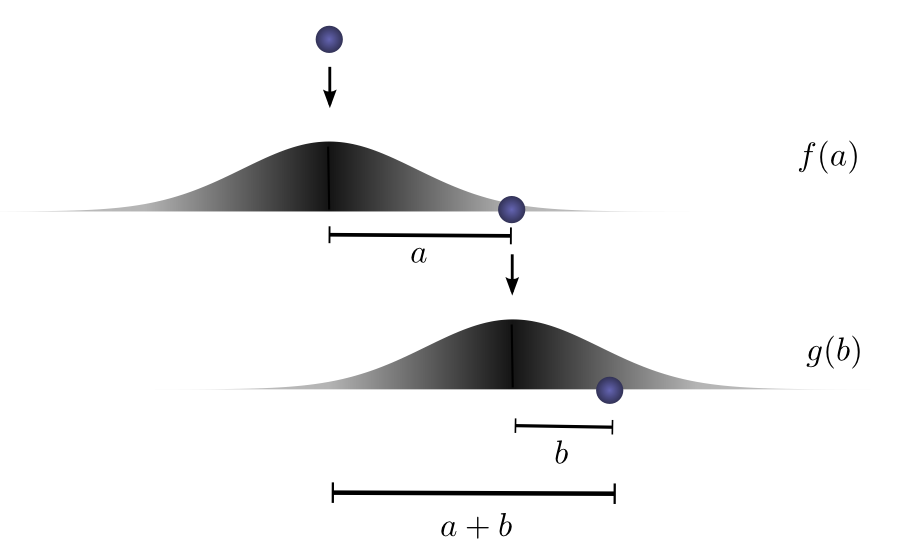
If we fix the result of the first drop so we know the ball went distance aa, for the ball to go a total distance cc, the distance traveled in the second drop is also fixed at bb, where a+b=cabc. So the probability of this happening is simply f(a)⋅g(b)fagb.1

Let’s think about this with a specific discrete example. We want the total distance cc to be 3. If the first time it rolls, a=2a2, the second time it must roll b=1b1 in order to reach our total distance a+b=3ab3. The probability of this is f(2)⋅g(1)f2g1.

However, this isn’t the only way we could get to a total distance of 3. The ball could roll 1 units the first time, and 2 the second. Or 0 units the first time and all 3 the second. It could go any aaand bb, as long as they add to 3.

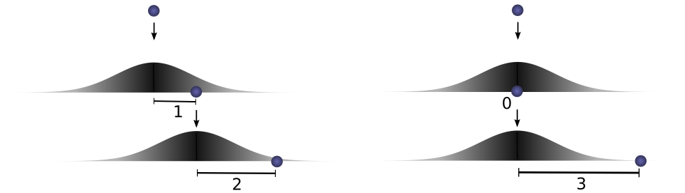
The probabilities are f(1)⋅g(2)f1g2 and f(0)⋅g(3)f0g3, respectively.

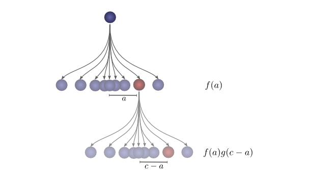
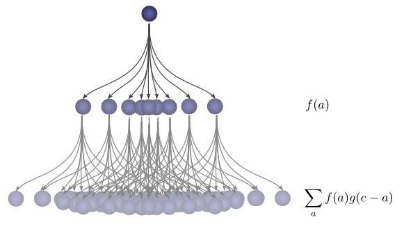
In order to find the total likelihood of the ball reaching a total distance of cc, we can’t consider only one possible way of reaching cc. Instead, we consider all the possible ways of partitioning ccinto two drops aa and bb and sum over the probability of each way.

...  f(0)⋅g(3) + f(1)⋅g(2) + f(2)⋅g(1)  ...  f0g3  f1g2  f2g1  

We already know that the probability for each case of a+b=cabc is simply f(a)⋅g(b)fagb. So, summing over every solution to a+b=cabc, we can denote the total likelihood as:

∑a+b=cf(a)⋅g(b)abcfagb

Turns out, we’re doing a convolution! In particular, the convolution of ff and gg, evluated at cc is defined:

(f∗g)(c)=∑a+b=cf(a)⋅g(b)    fgcabcfagb    

If we substitute b=c−abca, we get:

(f∗g)(c)=∑af(a)⋅g(c−a)fgcafagca

This is the standard definition2 of convolution.

To make this a bit more concrete, we can think about this in terms of positions the ball might land. After the first drop, it will land at an intermediate position aa with probability f(a)fa. If it lands at aa, it has probability g(c−a)gca of landing at a position cc.

To get the convolution, we consider all intermediate positions.

Visualizing Convolutions

There’s a very nice trick that helps one think about convolutions more easily.

First, an observation. Suppose the probability that a ball lands a certain distance xx from where it started is f(x)fx. Then, afterwards, the probability that it started a distance xx from where it landed is f(−x)fx.

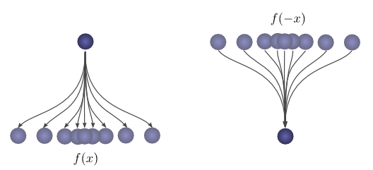
If we know the ball lands at a position cc after the second drop, what is the probability that the previous position was aa?

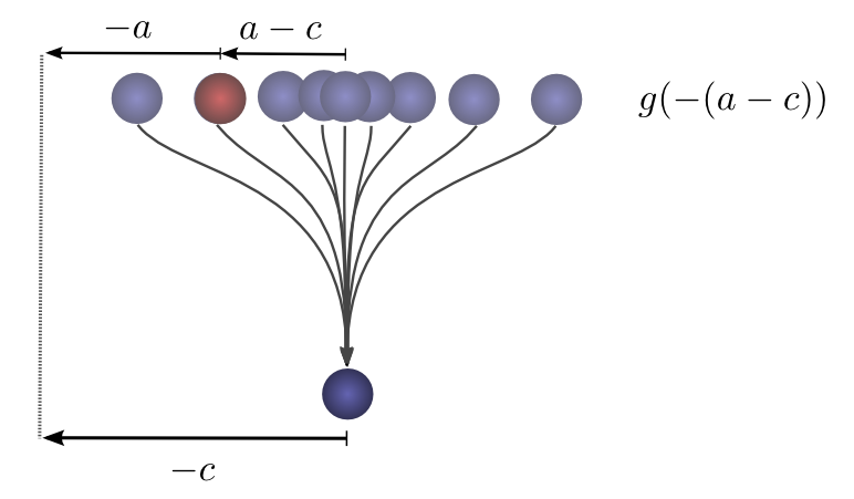
So the probability that the previous position was aa is g(−(a−c))=g(c−a)gacgca.

Now, consider the probability each intermediate position contributes to the ball finally landing at cc. We know the probability of the first drop putting the ball into the intermediate position a is f(a)fa. We also know that the probability of it having been in aa, if it lands at cc is g(c−a)gca.

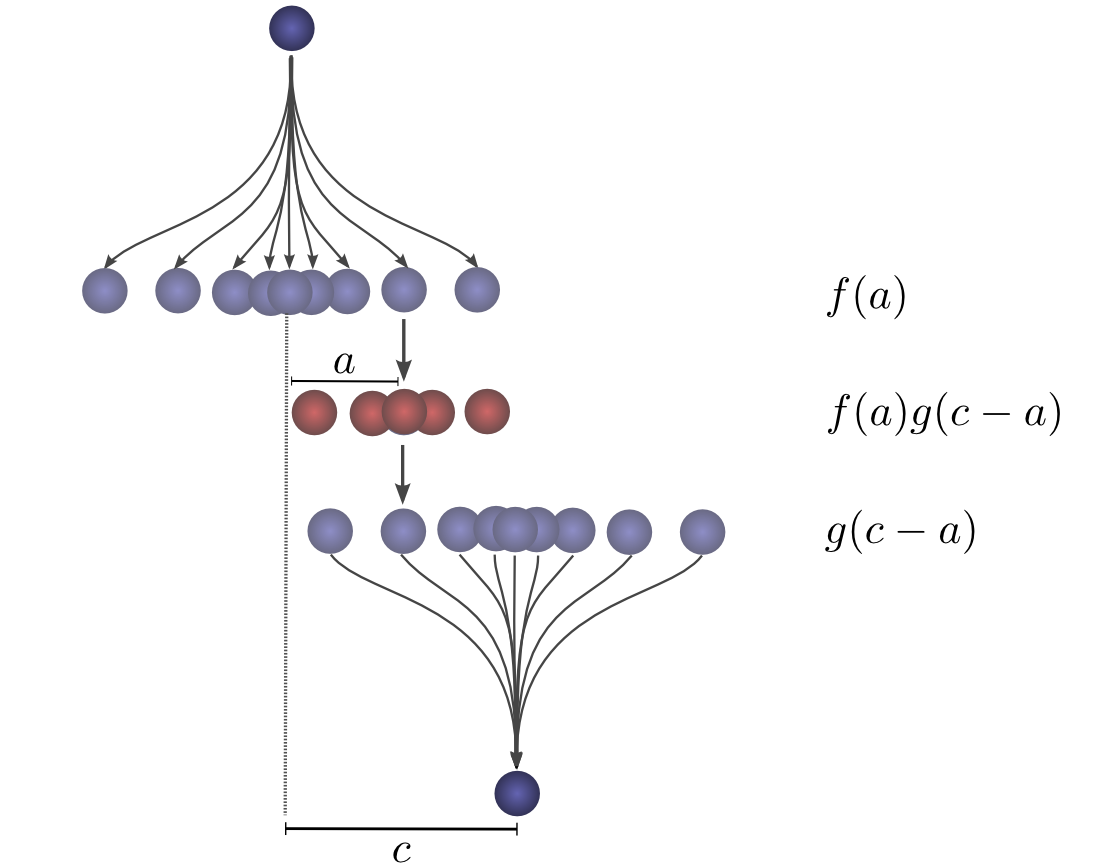
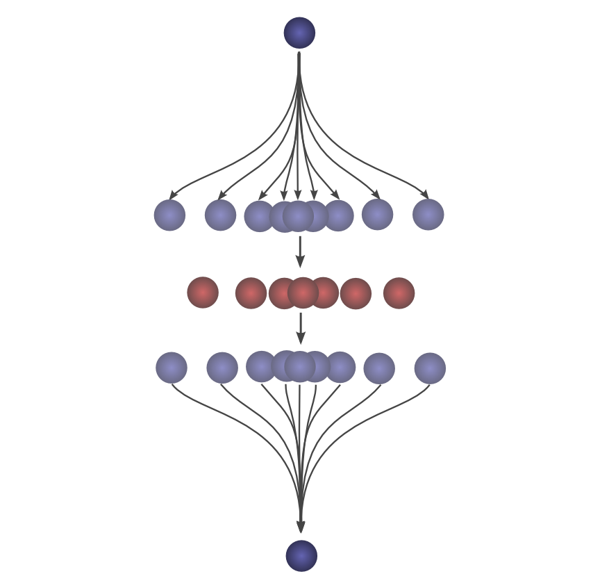
Summing over the aas, we get the convolution.

The advantage of this approach is that it allows us to visualize the evaluation of a convolution at a value cc in a single picture. By shifting the bottom half around, we can evaluate the convolution at other values of cc. This allows us to understand the convolution as a whole.

For example, we can see that it peaks when the distributions align.

And shrinks as the intersection between the distributions gets smaller.

By using this trick in an animation, it really becomes possible to visually understand convolutions.

Below, we’re able to visualize the convolution of two box functions:

From Wikipedia

Armed with this perspective, a lot of things become more intuitive.

Let’s consider a non-probabilistic example. Convolutions are sometimes used in audio manipulation. For example, one might use a function with two spikes in it, but zero everywhere else, to create an echo. As our double-spiked function slides, one spike hits a point in time first, adding that signal to the output sound, and later, another spike follows, adding a second, delayed copy.

2.CNN:笔记通俗理解卷积神经网络

 sigmoid的函数表达式如下

    其中z是一个线性组合，比如z可以等于：b + * + *。通过代入很大的正数或很小的负数到g(z)函数中可知，其结果趋近于0或1。

    因此，sigmoid函数g(z)的图形表示如下（ 横轴表示定义域z，纵轴表示值域g(z) ）：

    也就是说，sigmoid函数的功能是相当于把一个实数压缩至0到1之间。当z是非常大的正数时，g(z)会趋近于1，而z是非常大的负数时，则g(z)会趋近于0。

    压缩至0到1有何用处呢？用处是这样一来便可以把激活函数看作一种“分类的概率”，比如激活函数的输出为0.9的话便可以解释为90%的概率为正样本。

    举个例子，如下图（图引自Stanford机器学习公开课）

    z = b + * + *，其中b为偏置项 假定取-30，、都取为20

• 如果 = 0  = 0，则z = -30，g(z) = 1/( 1 + e^-z )趋近于0。此外，从上图sigmoid函数的图形上也可以看出，当z=-30的时候，g(z)的值趋近于0
• 如果 = 0  = 1，或 =1  = 0，则z = b + * + * = -30 + 20 = -10，同样，g(z)的值趋近于0
• 如果 = 1  = 1，则z = b + * + * = -30 + 20*1 + 20*1 = 10，此时，g(z)趋近于1。

    换言之，只有和都取1的时候，g(z)→1，判定为正样本；或取0的时候，g(z)→0，判定为负样本，如此达到分类的目的。

CNN之卷积计算层

4.1 什么是卷积

    首先，我们来了解下什么是卷积操作。

    对图像（不同的数据窗口数据）和滤波矩阵（一组固定的权重：因为每个神经元的权重固定，所以又可以看做一个恒定的滤波器filter）做内积（逐个元素相乘再求和）的操作就是所谓的『卷积』操作，也是卷积神经网络的名字来源。

    比如下图中，图中左边部分是原始输入数据，图中中间部分是滤波器filter，图中右边是输出的新的二维数据。

    分解下上图

对应位置上是数字先相乘后相加=

    中间滤波器filter与数据窗口做内积，其具体计算过程则是：4*0 + 0*0 + 0*0 + 0*0 + 0*1 + 0*1 + 0*0 + 0*1 + -4*2 = -8

4.2 图像上的卷积

    在计算过程中，输入是一定区域大小(width*height)的数据，和滤波器filter（一组固定的权重）做内积后等到新的二维数据。

    对于下图中，左边是图像输入，中间部分就是滤波器filter（一组固定的权重），不同的滤波器filter会得到不同的输出数据，比如颜色深浅、轮廓。相当于如果想提取图像的不同特征，则用不同的滤波器filter，提取想要的关于图像的特定信息：颜色深浅或轮廓。

    如下图所示

  

4.3 GIF动态卷积图

    在CNN中，滤波器filter对局部输入数据进行卷积计算。每计算完一个数据窗口内的局部数据后，数据窗口不断平移滑动，直到计算完所有数据。这个过程中，有这么几个参数： 
　　a. 深度depth：神经元个数，决定输出的depth厚度。 
　　b. 步长stride：决定滑动多少步可以到边缘 
　　c. 填充值zero-padding：在外围边缘补充若干圈0，方便从初始位置以步长为单位可以刚好滑倒末尾位置，通俗地讲就是为了总长能被步长整除。 

　　 

    cs231n课程中有一张卷积动图，貌似是用d3js 和一个util 画的，我根据cs231n的卷积动图依次截取了18张图，然后用一gif 制图工具制作了一gif 动态卷积图。如下gif 图所示，可以看到：

• 两个神经元，即depth=2
• 数据窗口每次移动两个步长取3*3的局部数据，即stride=2
• zero-padding=1

    然后分别以两个滤波器filter为轴滑动数组进行卷积计算，得到两组不同的结果。

    如果初看此图，可能不一定能立马理解啥意思，但结合上文的内容后，理解这个动图已经不是很困难的事情：左边是输入，中间部分是两个不同的滤波器Filter w0、Filter w1，最右边则是两个不同的输出。

    随着左边数据窗口的平移滑动，滤波器Filter w0 / Filter w1对不同的局部数据进行卷积计算。

    值得一提的是：

• 左边数据在变化，每次滤波器都是针对某一局部的数据窗口进行卷积，这就是所谓的CNN中的局部感知机制。
  
• 与此同时，数据窗口滑动，但中间滤波器Filter w0的权重（即每个神经元连接数据窗口的权重）是固定不变的，这个权重不变即所谓的CNN中的参数（权重）共享机制。

    我第一次看到上面这个动态图的时候，只觉得很炫，另外就是据说计算过程是“相乘后相加”，但到底具体是个怎么相乘后相加的计算过程 则无法一眼看出，网上也没有一目了然的计算过程。本文来细究下。

    首先，我们来分解下上述动图，如下图

    接着，我们细究下上图的具体计算过程。即上图中的输出结果-1具体是怎么计算得到的呢？其实，类似wx + b，w对应滤波器Filter w0，x对应不同的数据窗口，b对应Bias b0，相当于滤波器Filter w0与一个个数据窗口相乘再求和后，最后加上Bias b0得到输出结果-1，如下过程所示：

1* 0 + 1*0 + -1*0 

+

-1*0 + 0*0 + 1*1

+

-1*0 + -1*0 + 0*1

+

-1*0 + 0*0 + -1*0

+

0*0 + 0*1 + -1*1

+

1*0 + -1*0 + 0*2

+

0*0 + 1*0 + 0*0

+

1*0 + 0*2 + 1*0

+

0*0 + -1*0 + 1*0

+

 

1

=

1

    然后滤波器Filter w0固定不变，数据窗口向右移动2步，继续做内积计算，得到0的输出结果

    最后，换做另外一个不同的滤波器Filter w1、不同的偏置Bias b1，再跟图中最左边的数据窗口做卷积，可得到另外一个不同的输出。

CS231n课程笔记翻译：卷积神经网络笔记

参数共享：在卷积层中使用参数共享是用来控制参数的数量。就用上面的例子，在第一个卷积层就有55x55x96=290,400个神经元，每个有11x11x3=364个参数和1个偏差。将这些合起来就是290400x364=105,705,600个参数。单单第一层就有这么多参数，显然这个数目是非常大的。

作一个合理的假设：如果一个特征在计算某个空间位置(x,y)的时候有用，那么它在计算另一个不同位置(x2,y2)的时候也有用。基于这个假设，可以显著地减少参数数量。换言之，就是将深度维度上一个单独的2维切片看做深度切片（depth slice），比如一个数据体尺寸为[55x55x96]的就有96个深度切片，每个尺寸为[55x55]。在每个深度切片上的神经元都使用同样的权重和偏差。在这样的参数共享下，例子中的第一个卷积层就只有96个不同的权重集了，一个权重集对应一个深度切片，共有96x11x11x3=34,848个不同的权重，或34,944个参数（+96个偏差）。在每个深度切片中的55x55个权重使用的都是同样的参数。在反向传播的时候，都要计算每个神经元对它的权重的梯度，但是需要把同一个深度切片上的所有神经元对权重的梯度累加，这样就得到了对共享权重的梯度。这样，每个切片只更新一个权重集。

注意，如果在一个深度切片中的所有权重都使用同一个权重向量，那么卷积层的前向传播在每个深度切片中可以看做是在计算神经元权重和输入数据体的卷积（这就是“卷积层”名字由来）。这也是为什么总是将这些权重集合称为滤波器（filter）（或卷积核（kernel）），因为它们和输入进行了卷积。

局部连接：在处理图像这样的高维度输入时，让每个神经元都与前一层中的所有神经元进行全连接是不现实的。相反，我们让每个神经元只与输入数据的一个局部区域连接。该连接的空间大小叫做神经元的感受野（receptive field），它的尺寸是一个超参数（其实就是滤波器的空间尺寸）。在深度方向上，这个连接的大小总是和输入量的深度相等。需要再次强调的是，我们对待空间维度（宽和高）与深度维度是不同的：连接在空间（宽高）上是局部的，但是在深度上总是和输入数据的深度一致。

形象理解权值共享就是说：对输入图像，采用一个滤波核去扫这张图，在滑动卷积的时候，这个滤波器的参数是不变的，权重是一样的，即整幅图像共享一组权值。