Vehicle tracking using a support vector machine vs. YOLO

转载自：https://medium.com/@ksakmann/vehicle-detection-and-tracking-using-hog-features-svm-vs-yolo-73e1ccb35866?spm=5176.100239.0.0.g3fCcC#.9efrpug66

Introduction

The vehicle detection and tracking project of the Udacity Self-Driving Car Nanodegree is a challenge to apply traditional computer vision techniques, such as Histogram of Oriented Gradients (HOG) and other features combined with sliding windows to track vehicles in a video. The ideal solution would run in real-time, i.e. >30FPS. My go at a solution follows the 2005 approach byDalal and Triggs using a linear SVM and processes video at a measly 3FPS on an i7 CPU. Check thisrepo for the code and a more technical discussion.

<img class="progressiveMedia-noscript js-progressiveMedia-inner" src="https://cdn-images-1.medium.com/max/800/1*sbGY0u0OkjIkyujp5LN5rg.png">

YOLO applied to the Udacity vehicle tracking project video does an excellent job at detecting vehicles.

For fun I also passed the project video throughYOLO, a blazingly fast convolutional neural network for object detection. If you are working on a fast GPU (a GTX 1080 in my case) the video gets processed at about 65FPS. Yes! That’s more than 20x faster which is why I made no attempt at vectorizing my SVM+HOG solution. Although there certainly are opportunities, particularly the sliding windows part. I’ll discuss the YOLO results further down.

Data sets

I used the KITTI and GTI data sets as well as the Extra data that comes along with the project repository for training. There are only two classes: “cars” and “notcars”. The GTI data is taken from video streams. Therefore blindly randomizing all images and subsequently splitting into train and test sets introduces correlations between training and test sets. I therefore simply split off the final 30% of each data source as validation and test sets. All images (including ones with non-square aspect ratios) are resized to 64x64 pixels for feature extraction.

Feature Extraction

As a feature vector I used a combination of

• spatial features, which are nothing else but a down sampled copy of the image patch to be checked itself (16x16 pixels)
• color histogram features that capture the statistical color information of each image patch. Cars often come in very saturated colors which is captured by this part of the feature vector.
• Histogram of oriented gradients (HOG) features, that capture the gradient structure of each image channel and work well under different lighting conditions

You can read more about HOG features in thisblog post, but the idea is to make the feature vector more robust to variations of perspective and illumination by aggregating the gradients on an image in a histogram.
Here is a visualization of what HOG features look like for “cars” and “notcars” images.

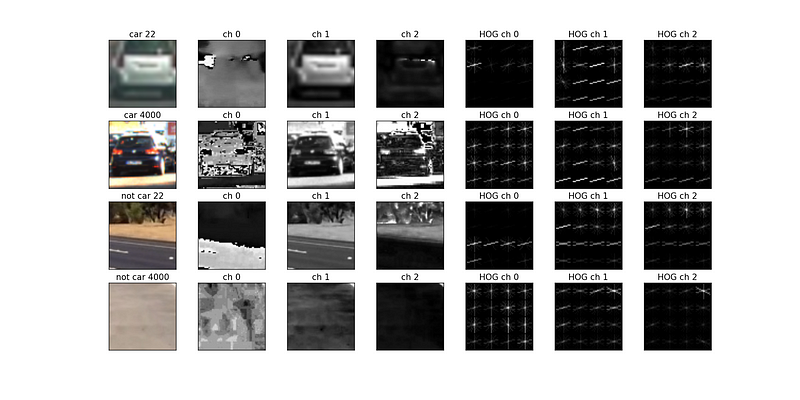
HOG features.First four columns from the left: typical examples of training data and their channels in HLS color space. Rightmost three columns: visualization of the HOG vectors for each channel.

The final feature vector contains features extracted in the three different ways quoted above. It is therefore necessary to scale every feature to prevent one of the features being dominant merely due to its value range being at a different scale. I therefore used the Standard.Scaler function of the scikit learn package to standardize features by removing the mean and scaling to unit variance.

Training a linear support vector machine

Unlike many other classification or detection problems there is a strong real-time requirement for detecting cars. So a trade-off between high accuracy and speed is unavoidable. The two main parameters that influence the performance are the length of the feature vector and the algorithm for detecting the vehicles. A linear SVM offered the best compromise between speed and accuracy, outperforming random forests (fast, but less accurate) and nonlinear SVMs (rbf kernel, very slow). The final test accuracy using a feature vector containing 6156 features was above 98.5% which sounds good, but is much less so when you find out that those remaining 1.5% are frequently appearing image patches, particularly lane lines, crash barriers and guard rails.

False Positives: frequently appearing image patches still get misclassified, despite 98.5% test accuracy.

Sliding windows

In the standard vehicle detection approach the frames recorded by a video camera the image is scanned using a sliding window. For every window the feature vector is computed and fed into the classifier. As the cars appear at different distances, it is also necessary to search at several scales. Commonly over a hundred feature vectors need to be extracted and fed into the classifier for every single frame. Fortunately this part can be vectorized (not done). Shown below is a typical example of positive detections together with all ~150 windows that are used for detecting cars. As expected there are some false positives.

For filtering out the false positives I always kept track of the detected windows of the last 30 frames and only considered those parts of the image as positives where more than 15 detections had been recorded. The result is a heatmap with significantly reduced noise, as shown below

Left:All detected windows of a frame.Right:heatmap of the last 30 frames.

From the thresholding heatmap the final bounding boxes are determined as the smallest rectangular box that contains all nonzero values of the heatmap

Left:binarized heatmap thresholded at 15 detections.Right:final result of drawn bounding boxes.

Applying the entire pipeline to a video results in bounding boxes drawn around the cars, as shown here:Comparison to YOLO and Conclusions

The above pipeline using HOG features and a linear SVM is well-known since 2005. Very recently extremely fast neural network based object detectors have emerged which allow object detection faster than realtime. I merely cloned the original darknet repository and applied YOLO to the project video. I only needed to do a minor code modification to allow saving videos directly. The result is quite amazing. As no sliding windows are used the detection is extremely fast. A frame is passed to the network and processed precisely once, hence the name YOLO — “you only look once”.

YOLO applied to the project video

A forward pass of an entire image through the network is more expensive than extracting a feature vector of an image patch and passing it through an SVM. Hoever, this operation needs to be done exactly once for an entire image, as opposed to the roughly 150 times in the SVM+HOG approach. For generating the video above I did no performance optimization, like reducing the image or defining a region of interest, or even training specifically for cars. Nevertheless, YOLO is more than 20x faster than the SVM+HOG and at least as accurate. The detection threshold can be set to any confidence level. Here I left it at the default of 50% and at no time were any objects other than cars detected (OK, one time a car was confused for a truck). Note that there are many more classes, like “person”, “cell phone”,”dog” and others. So not only the false positive rate, but also the false negative rate was very good. I find this extremely exciting and will check the possibilities for vehicle detection further in a separate project. This will be fun.

Thanks for reading,