Reinforcement Learning (DQN) tutorial

Author: Adam Paszke

This tutorial shows how to use PyTorch to train a Deep Q Learning (DQN) agent on the CartPole-v0 task from the OpenAI Gym.

Task

The agent has to decide between two actions - moving the cart left or right - so that the pole attached to it stays upright. You can find an official leaderboard with various algorithms and visualizations at the Gym website.

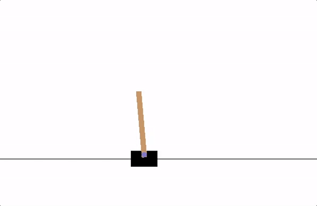
cartpole

As the agent observes the current state of the environment and chooses an action, the environmenttransitions to a new state, and also returns a reward that indicates the consequences of the action. In this task, the environment terminates if the pole falls over too far.

The CartPole task is designed so that the inputs to the agent are 4 real values representing the environment state (position, velocity, etc.). However, neural networks can solve the task purely by looking at the scene, so we’ll use a patch of the screen centered on the cart as an input. Because of this, our results aren’t directly comparable to the ones from the official leaderboard - our task is much harder. Unfortunately this does slow down the training, because we have to render all the frames.

Strictly speaking, we will present the state as the difference between the current screen patch and the previous one. This will allow the agent to take the velocity of the pole into account from one image.

Packages

First, let’s import needed packages. Firstly, we need gym for the environment (Install using pip install gym). We’ll also use the following from PyTorch:

• neural networks (torch.nn)
• optimization (torch.optim)
• automatic differentiation (torch.autograd)
• utilities for vision tasks (torchvision - a separate package).

import gymimport mathimport randomimport numpy as npimport matplotlibimport matplotlib.pyplot as pltfrom collections import namedtuplefrom itertools import countfrom copy import deepcopyfrom PIL import Imageimport torchimport torch.nn as nnimport torch.optim as optimimport torch.autograd as autogradimport torch.nn.functional as Fimport torchvision.transforms as Tenv = gym.make('CartPole-v0')is_ipython = 'inline' in matplotlib.get_backend()if is_ipython:    from IPython import display

Replay Memory

We’ll be using experience replay memory for training our DQN. It stores the transitions that the agent observes, allowing us to reuse this data later. By sampling from it randomly, the transitions that build up a batch are decorrelated. It has been shown that this greatly stabilizes and improves the DQN training procedure.

For this, we’re going to need two classses:

• Transition - a named tuple representing a single transition in our environment
• ReplayMemory - a cyclic buffer of bounded size that holds the transitions observed recently. It also implements a .sample() method for selecting a random batch of transitions for training.

Transition = namedtuple('Transition',                        ('state', 'action', 'next_state', 'reward'))class ReplayMemory(object):    def __init__(self, capacity):        self.capacity = capacity        self.memory = []        self.position = 0    def push(self, *args):        """Saves a transition."""        if len(self.memory) < self.capacity:            self.memory.append(None)        self.memory[self.position] = Transition(*args)        self.position = (self.position + 1) % self.capacity    def sample(self, batch_size):        return random.sample(self.memory, batch_size)    def __len__(self):        return len(self.memory)

Now, let’s define our model. But first, let quickly recap what a DQN is.

DQN algorithm

Our environment is deterministic, so all equations presented here are also formulated deterministically for the sake of simplicity. In the reinforcement learning literature, they would also contain expectations over stochastic transitions in the environment.

Our aim will be to train a policy that tries to maximize the discounted, cumulative reward Rt0=∑∞t=t0γt−t0rtRt0=∑t=t0∞γt−t0rt, where Rt0Rt0 is also known as the return. The discount, γγ, should be a constant between 00 and 11 that ensures the sum converges. It makes rewards from the uncertain far future less important for our agent than the ones in the near future that it can be fairly confident about.

The main idea behind Q-learning is that if we had a function Q∗:State×Action→RQ∗:State×Action→R, that could tell us what our return would be, if we were to take an action in a given state, then we could easily construct a policy that maximizes our rewards:

π∗(s)=argmaxa Q∗(s,a)π∗(s)=argmaxa Q∗(s,a)

However, we don’t know everything about the world, so we don’t have access to Q∗Q∗. But, since neural networks are universal function approximators, we can simply create one and train it to resemble Q∗Q∗.

For our training update rule, we’ll use a fact that every QQ function for some policy obeys the Bellman equation:

Qπ(s,a)=r+γQπ(s′,π(s′))Qπ(s,a)=r+γQπ(s′,π(s′))

The difference between the two sides of the equality is known as the temporal difference error, δδ:

δ=Q(s,a)−(r+γmaxaQ(s′,a))δ=Q(s,a)−(r+γmaxaQ(s′,a))

To minimise this error, we will use the Huber loss. The Huber loss acts like the mean squared error when the error is small, but like the mean absolute error when the error is large - this makes it more robust to outliers when the estimates of QQ are very noisy. We calculate this over a batch of transitions, BB, sampled from the replay memory:

L=1|B|∑(s,a,s′,r) ∈ BL(δ)L=1|B|∑(s,a,s′,r) ∈ BL(δ)

whereL(δ)={12δ2|δ|−12for |δ|≤1,otherwise.whereL(δ)={12δ2for |δ|≤1,|δ|−12otherwise.

Q-network

Our model will be a convolutional neural network that takes in the difference between the current and previous screen patches. It has two outputs, representing Q(s,left)Q(s,left) and Q(s,right)Q(s,right) (where ssis the input to the network). In effect, the network is trying to predict the quality of taking each action given the current input.

class DQN(nn.Module):    def __init__(self):        super(DQN, self).__init__()        self.conv1 = nn.Conv2d(3, 16, kernel_size=5, stride=2)        self.bn1 = nn.BatchNorm2d(16)        self.conv2 = nn.Conv2d(16, 32, kernel_size=5, stride=2)        self.bn2 = nn.BatchNorm2d(32)        self.conv3 = nn.Conv2d(32, 32, kernel_size=5, stride=2)        self.bn3 = nn.BatchNorm2d(32)        self.head = nn.Linear(448, 2)    def forward(self, x):        x = F.relu(self.bn1(self.conv1(x)))        x = F.relu(self.bn2(self.conv2(x)))        x = F.relu(self.bn3(self.conv3(x)))        return self.head(x.view(x.size(0), -1))

Input extraction

The code below are utilities for extracting and processing rendered images from the environment. It uses the torchvision package, which makes it easy to compose image transforms. Once you run the cell it will display an example patch that it extracted.

resize = T.Compose([T.ToPILImage(),                    T.Scale(40, interpolation=Image.CUBIC),                    T.ToTensor()])# This is based on the code from gym.screen_width = 600def get_cart_location():    world_width = env.x_threshold * 2    scale = screen_width / world_width    return int(env.state[0] * scale + screen_width / 2.0)  # MIDDLE OF CARTdef get_screen():    screen = env.render(mode='rgb_array').transpose(        (2, 0, 1))  # transpose into torch order (CHW)    # Strip off the top and bottom of the screen    screen = screen[:, 160:320]    view_width = 320    cart_location = get_cart_location()    if cart_location < view_width // 2:        slice_range = slice(view_width)    elif cart_location > (screen_width - view_width // 2):        slice_range = slice(-view_width, None)    else:        slice_range = slice(cart_location - view_width // 2,                            cart_location + view_width // 2)    # Strip off the edges, so that we have a square image centered on a cart    screen = screen[:, :, slice_range]    # Convert to float, rescare, convert to torch tensor    # (this doesn't require a copy)    screen = np.ascontiguousarray(screen, dtype=np.float32) / 255    screen = torch.from_numpy(screen)    # Resize, and add a batch dimension (BCHW)    return resize(screen).unsqueeze(0)env.reset()plt.imshow(get_screen().squeeze(0).permute(    1, 2, 0).numpy(), interpolation='none')plt.show()

Training

Hyperparameters and utilities

This cell instantiates our model and its optimizer, and defines some utilities:

• Variable - this is a simple wrapper around torch.autograd.Variable that will automatically send the data to the GPU every time we construct a Variable.
• select_action - will select an action accordingly to an epsilon greedy policy. Simply put, we’ll sometimes use our model for choosing the action, and sometimes we’ll just sample one uniformly. The probability of choosing a random action will start at EPS_START and will decay exponentially towards EPS_END. EPS_DECAY controls the rate of the decay.
• plot_durations - a helper for plotting the durations of episodes, along with an average over the last 100 episodes (the measure used in the official evaluations). The plot will be underneath the cell containing the main training loop, and will update after every episode.

BATCH_SIZE = 128GAMMA = 0.999EPS_START = 0.9EPS_END = 0.05EPS_DECAY = 200USE_CUDA = torch.cuda.is_available()model = DQN()memory = ReplayMemory(10000)optimizer = optim.RMSprop(model.parameters())if USE_CUDA:    model.cuda()class Variable(autograd.Variable):    def __init__(self, data, *args, **kwargs):        if USE_CUDA:            data = data.cuda()        super(Variable, self).__init__(data, *args, **kwargs)steps_done = 0def select_action(state):    global steps_done    sample = random.random()    eps_threshold = EPS_END + (EPS_START - EPS_END) * \        math.exp(-1. * steps_done / EPS_DECAY)    steps_done += 1    if sample > eps_threshold:        return model(Variable(state, volatile=True)).data.max(1)[1].cpu()    else:        return torch.LongTensor([[random.randrange(2)]])episode_durations = []def plot_durations():    plt.figure(1)    plt.clf()    durations_t = torch.Tensor(episode_durations)    plt.xlabel('Episode')    plt.ylabel('Duration')    plt.plot(durations_t.numpy())    # Take 100 episode averages and plot them too    if len(durations_t) >= 100:        means = durations_t.unfold(0, 100, 1).mean(1).view(-1)        means = torch.cat((torch.zeros(99), means))        plt.plot(means.numpy())    if is_ipython:        display.clear_output(wait=True)        display.display(plt.gcf())

Training loop

Finally, the code for training our model.

Here, you can find an optimize_model function that performs a single step of the optimization. It first samples a batch, concatenates all the tensors into a single one, computes Q(st,at)Q(st,at) and V(st+1)=maxaQ(st+1,a)V(st+1)=maxaQ(st+1,a), and combines them into our loss. By defition we set V(s)=0V(s)=0 if ss is a terminal state.

last_sync = 0def optimize_model():    global last_sync    if len(memory) < BATCH_SIZE:        return    transitions = memory.sample(BATCH_SIZE)    # Transpose the batch (see http://stackoverflow.com/a/19343/3343043 for    # detailed explanation).    batch = Transition(*zip(*transitions))    # Compute a mask of non-final states and concatenate the batch elements    non_final_mask = torch.ByteTensor(        tuple(map(lambda s: s is not None, batch.next_state)))    if USE_CUDA:        non_final_mask = non_final_mask.cuda()    # We don't want to backprop through the expected action values and volatile    # will save us on temporarily changing the model parameters'    # requires_grad to False!    non_final_next_states = Variable(torch.cat([s for s in batch.next_state                                                if s is not None]),                                     volatile=True)    state_batch = Variable(torch.cat(batch.state))    action_batch = Variable(torch.cat(batch.action))    reward_batch = Variable(torch.cat(batch.reward))    # Compute Q(s_t, a) - the model computes Q(s_t), then we select the    # columns of actions taken    state_action_values = model(state_batch).gather(1, action_batch)    # Compute V(s_{t+1}) for all next states.    next_state_values = Variable(torch.zeros(BATCH_SIZE))    next_state_values[non_final_mask] = model(non_final_next_states).max(1)[0]    # Now, we don't want to mess up the loss with a volatile flag, so let's    # clear it. After this, we'll just end up with a Variable that has    # requires_grad=False    next_state_values.volatile = False    # Compute the expected Q values    expected_state_action_values = (next_state_values * GAMMA) + reward_batch    # Compute Huber loss    loss = F.smooth_l1_loss(state_action_values, expected_state_action_values)    # Optimize the model    optimizer.zero_grad()    loss.backward()    for param in model.parameters():        param.grad.data.clamp_(-1, 1)    optimizer.step()

Below, you can find the main training loop. At the beginning we reset the environment and initialize the state variable. Then, we sample an action, execute it, observe the next screen and the reward (always 1), and optimize our model once. When the episode ends (our model fails), we restart the loop.

Below, num_episodes is set small. You should download the notebook and run lot more epsiodes.

num_episodes = 10for i_episode in range(num_episodes):    # Initialize the environment and state    env.reset()    last_screen = get_screen()    current_screen = get_screen()    state = current_screen - last_screen    for t in count():        # Select and perform an action        action = select_action(state)        _, reward, done, _ = env.step(action[0, 0])        reward = torch.Tensor([reward])        # Observe new state        last_screen = current_screen        current_screen = get_screen()        if not done:            next_state = current_screen - last_screen        else:            next_state = None        # Store the transition in memory        memory.push(state, action, next_state, reward)        # Move to the next state        state = next_state        # Perform one step of the optimization (on the target network)        optimize_model()        if done:            episode_durations.append(t + 1)            plot_durations()            break

Total running time of the script: ( 0 minutes 0.000 seconds)