[DL]1.开始学习TensorFlow

原文链接

---

开始学习TensorFlow

在学习本文之前，需要首先安装Tensorflow。本文介绍以下知识：

• 如何使用Python编程
• 关于矩阵的一些知识
• 关于机器学习的一些知识

TensorFlow提供多种多样的API。最底层的API是Tensorflow Core，提供完全的程序控制。我们推荐机器学习研究者以及其他想要对他们的模型有更良好的控制能力的这类人使用TensorFLow Core。更高级的API是构建在Tensorflow Core基础之上的。这些更高等级的API减少重复性工作并且能在不同的用户之间保持一致性。比如tf.contrib.learn协助管理数据集，估计，训练和接口。值得注意的是一些高等级的API方法名字包含contrib的是在开发版本。这意味着一些contrib方法有可能在接下来的版本中过时或者改变。
本文使用Tensorflow Core作为入门。接着介绍了如何使用tf.contrib.learn实现相同的模型。了解Tensorflow Core的规则将使得你能够在心里明白使用更高级的API时模型内部是如何工作的。

张量（Tensor）

tensor（张量）是TensorFlow中数据的中心单元。张量由原始值的集合组成通过变形为多维矩阵。张量的等级是它的维度数量。这里给出部分示例：

3 # 0 tensor[1. ,2., 3.] # 1 tensor 3维[[1., 2., 3.], [4., 5., 6.]] # 2 tensor   2*3维[[[1., 2., 3.]], [[7., 8., 9.]]] # 3 tensor 2*1*3维

TensorFlow Core 教程

导入 TensorFlow

tensorFlow的import表达式一般长这个样子：

import tensorflow as tf

import之后，就可以调用所有的TensorFlow类，方法，符号了。

The Computational Graph

TensorFlow Core程序由两个分离的部分组成：

• 创建图
• 运行图

计算图（computational graph）将一系列的TensorFLow操作排列成图的节点。下面试着创建一个简单的图。每一个图有0个或者多个tensor输入，一个张量作为输出。节点的一种类型是常量，正如所有的TensorFlow常量一样，这个常量没有输入，输出的是它内部保存的值。下面创建了两个浮点型张量 node1和node2：

node1 = tf.constant(3.0, tf.float32)node2 = tf.constant(4.0) # also tf.float32 implicitlyprint(node1, node2)

输出：

Tensor("Const:0", shape=(), dtype=float32) Tensor("Const_1:0", shape=(), dtype=float32)

注意，这里的最终输出并不是3.4和4.0,而是当评估他们的时候将分别输出3.0和4.0.为了最终评估节点，必须在一个session里面运行图。一个session封装tensorflow运行时的控制和状态。

下面将创建一个sesion对象，之后调用它的run方法来通过运行图来评估node1和node2.如下演示了如何在session中运行图：

sess = tf.Session()print(sess.run([node1, node2]))

可以看到最终的输出是3.0 and 4.0:

[3.0, 4.0]

我们可以通过组合多个张量节点以及操作（操作也是节点）来完成更复杂的计算。比如，将两个常量节点相加，生成一个新的图：

node3 = tf.add(node1, node2)print("node3: ", node3)print("sess.run(node3): ",sess.run(node3))

最后两句表达式的输出如下：

node3:  Tensor("Add_2:0", shape=(), dtype=float32)sess.run(node3):  7.0

TensorFlow提供一个很实用的称为TensorBoard的工具，它可以可视化一个图。这里给出一个TensorBoard可视化图之后的结果：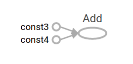

图中并没有什么特别值得注意的东西，因为它仅仅生成一个常量结果。图可以通过参数化来接受外部的输入，称为placeholder。一个placeholder预示着它将提供数值。

a = tf.placeholder(tf.float32)b = tf.placeholder(tf.float32)adder_node = a + b  #tf.add(a, b)的快速实现

上面的三行代码像一个方法或者lambda表达式，定义了两个输入以及一个操作。我们可以通过使用feed_dict为tensor中的placeholder指定输入参数来评估图。

print(sess.run(adder_node, {a: 3, b:4.5}))print(sess.run(adder_node, {a: [1,3], b: [2, 4]}))

输出为：

7.5[ 3.  7.]

在TensorBoard中显示如下：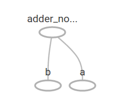

我们可以用图来完成更复杂的操作：

add_and_triple = adder_node * 3.print(sess.run(add_and_triple, {a: 3, b:4.5}))

输入如下：

22.5

在TensorBroad中如下所示：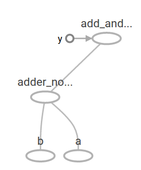

机器学习中，我们通常想要一个模型能够接受任意参数作为输入。为了使得模型可训练，我们需要修改图接收相同的输入产生新的输出。Variables允许我们给图添加可训练的参数，Variables仅通过初始值和类型构造：

W = tf.Variable([.3], tf.float32)b = tf.Variable([-.3], tf.float32)x = tf.placeholder(tf.float32)linear_model = W * x + b

常量在调用tf.constant方法的时候初始化，并且之后不能被改变。相反的，变量在调用tf.variable的时候没有初始化。在TensorFlow程序中为了初始化所有的变量需要通过如下的操作：

init = tf.global_variables_initializer()sess.run(init)

init是TensorFlow子图的一个操作，用来初始化所有的全局变量。直到调用了sess.run,变量才会被初始化。
既然x是一个placeholder，我们可以同时给x取多个值来评估linear_model。
print(sess.run(linear_model, {x:[1,2,3,4]}))
输出为：

[ 0.          0.30000001  0.60000002  0.90000004]

到这里，我们已经创建了一个模型，但是我们不知道他到底有多好。为了在训练数据基础上评估这个模型，我们需要一个placeholder类型的y来提供期望的数值，并且需要写一个损失函数。
损失函数当前模型输出距离提供的结果的误差有多大。我们将使用一个标准的线性回归损失模型：通过计算目标结果减去当前模型的结果的差值的平方的和。linear_model-y得到一个向量，向量的每一维都对应相应的误差。通过调用tf.square计算误差的平方。然后使用tf.reduce_sum把所有误差的平方相加得到一个单独标量表示所有的误差。

y = tf.placeholder(tf.float32)squared_deltas = tf.square(linear_model - y)loss = tf.reduce_sum(squared_deltas)print(sess.run(loss, {x:[1,2,3,4], y:[0,-1,-2,-3]}))

输出的误差为：

23.66

我们可以手动的改进这个模型，通过调整W为-1和b的值为1得到完美的结果。通过给tf.Variable声明的时候赋值来初始化一个变量，变量的值可以通过使用tf.assign操作来改变。比如W=-1和b=1就是这个模型最优的结果：

fixW = tf.assign(W, [-1.])fixb = tf.assign(b, [1.])sess.run([fixW, fixb])print(sess.run(loss, {x:[1,2,3,4], y:[0,-1,-2,-3]}))

最后的输出显示损失值为：

0.0

这里我们是通过猜测来找到W和b的值，但是在机器学习中找到正确的模型参数是自动进行的。本文将在接下来介绍如何实现。

tf.train API

TensorFlow提供优化器通过慢慢的改变每一个变量的值来最小化损失函数。最简单的优化器就是梯度下降,根据损失函数对变量求得的导数大小来改变每一个变量。TensorFlow能够使用tf.gradients方法对模型自动求导。简单的来说，优化器通常自动的完成这个任务，比如：

optimizer = tf.train.GradientDescentOptimizer(0.01)train = optimizer.minimize(loss)sess.run(init) # reset values to incorrect defaults.for i in range(1000):  sess.run(train, {x:[1,2,3,4], y:[0,-1,-2,-3]})print(sess.run([W, b]))

模型参数的结果:

[array([-0.9999969], dtype=float32), array([ 0.99999082], dtype=float32)]

以上就完成了简单的机器学习的线性回归的例子。TensotFlow通过少量的代码就完成了上述任务，当然了，复杂的模型和方法需要更多的代码。TensorFlow提供更高等级的共同模式，结构，方法的抽象。在接下来的章节将介绍这些。

完整的代码

import numpy as npimport tensorflow as tf# Model parametersW = tf.Variable([.3], tf.float32)b = tf.Variable([-.3], tf.float32)# Model input and outputx = tf.placeholder(tf.float32)linear_model = W * x + by = tf.placeholder(tf.float32)# lossloss = tf.reduce_sum(tf.square(linear_model - y)) # sum of the squares# optimizeroptimizer = tf.train.GradientDescentOptimizer(0.01)train = optimizer.minimize(loss)# training datax_train = [1,2,3,4]y_train = [0,-1,-2,-3]# training loopinit = tf.global_variables_initializer()sess = tf.Session()sess.run(init) # reset values to wrongfor i in range(1000):  sess.run(train, {x:x_train, y:y_train})# evaluate training accuracycurr_W, curr_b, curr_loss  = sess.run([W, b, loss], {x:x_train, y:y_train})print("W: %s b: %s loss: %s"%(curr_W, curr_b, curr_loss))

最后的输出如下：

W: [-0.9999969] b: [ 0.99999082] loss: 5.69997e-11

本例比之前的例子更复杂，但是也可以通过TensorFlowBroad可视化。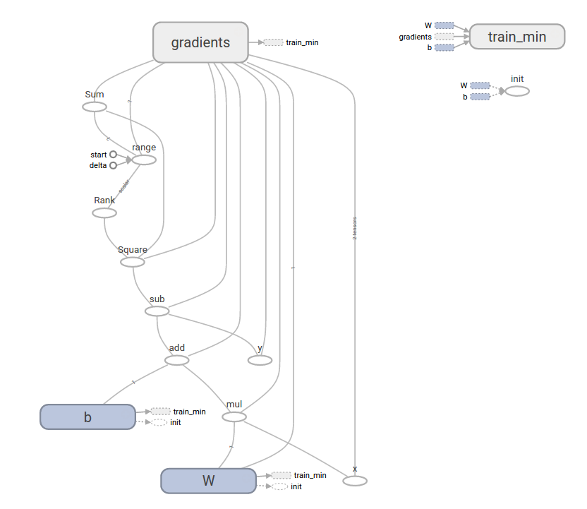

tf.contrib.learn

tf.contrib.learn是一个高等级的TensorFlow类，它使得机器学习变得简单，包括：

• 循环进行训练
• 循环进行评估
• 管理数据集
• 管理反馈

tf.contrib.learn定义了很多公共模型。

基本用法

tf.contrib.learn使得线性回归变得更加简单:

import tensorflow as tf# NumPy is often used to load, manipulate and preprocess data.import numpy as np# Declare list of features. We only have one real-valued feature. There are many# other types of columns that are more complicated and useful.features = [tf.contrib.layers.real_valued_column("x", dimension=1)]# An estimator is the front end to invoke training (fitting) and evaluation# (inference). There are many predefined types like linear regression,# logistic regression, linear classification, logistic classification, and# many neural network classifiers and regressors. The following code# provides an estimator that does linear regression.estimator = tf.contrib.learn.LinearRegressor(feature_columns=features)# TensorFlow provides many helper methods to read and set up data sets.# Here we use two data sets: one for training and one for evaluation# We have to tell the function how many batches# of data (num_epochs) we want and how big each batch should be.x_train = np.array([1., 2., 3., 4.])y_train = np.array([0., -1., -2., -3.])x_eval = np.array([2., 5., 8., 1.])y_eval = np.array([-1.01, -4.1, -7, 0.])input_fn = tf.contrib.learn.io.numpy_input_fn({"x":x_train}, y_train,                                              batch_size=4,                                              num_epochs=1000)eval_input_fn = tf.contrib.learn.io.numpy_input_fn(    {"x":x_eval}, y_eval, batch_size=4, num_epochs=1000)# We can invoke 1000 training steps by invoking the  method and passing the# training data set.estimator.fit(input_fn=input_fn, steps=1000)# Here we evaluate how well our model did.train_loss = estimator.evaluate(input_fn=input_fn)eval_loss = estimator.evaluate(input_fn=eval_input_fn)print("train loss: %r"% train_loss)print("eval loss: %r"% eval_loss)

最终的结果：

    {'global_step': 1000, 'loss': 1.9650059e-11}

自定义模型

tf.contrib.learn 并没有限定模型. 如果想要创建一个TensorFlow中没有创建的模型，我们依然可以保持tf.contrib.learn的高度抽象的数据集、反馈、训练等。接下来，我们将展示如何实现TensorFlow中LinearRegressor相等的模型，而仅仅使用TensorFlow 低等级API知识。

为了使用tf.contrib.learn定义一个自定义模型，我们需要使用的tf.contrib.learn.Estimator和tf.contrib.learn.LinearRegressor事实上是tf.contrib.learn.Estimator的一个子类。这里传递给Estimator一个函数模型model_fn声明 tf.contrib.learn需要如何评估预测, 训练步骤和损耗，而不是使用子类。代码如下：

import numpy as npimport tensorflow as tf# Declare list of features, we only have one real-valued featuredef model(features, labels, mode):  # Build a linear model and predict values  W = tf.get_variable("W", [1], dtype=tf.float64)  b = tf.get_variable("b", [1], dtype=tf.float64)  y = W*features['x'] + b  # Loss sub-graph  loss = tf.reduce_sum(tf.square(y - labels))  # Training sub-graph  global_step = tf.train.get_global_step()  optimizer = tf.train.GradientDescentOptimizer(0.01)  train = tf.group(optimizer.minimize(loss),                   tf.assign_add(global_step, 1))  # ModelFnOps connects subgraphs we built to the  # appropriate functionality.  return tf.contrib.learn.ModelFnOps(      mode=mode, predictions=y,      loss=loss,      train_op=train)estimator = tf.contrib.learn.Estimator(model_fn=model)# define our data setx = np.array([1., 2., 3., 4.])y = np.array([0., -1., -2., -3.])input_fn = tf.contrib.learn.io.numpy_input_fn({"x": x}, y, 4, num_epochs=1000)# trainestimator.fit(input_fn=input_fn, steps=1000)# evaluate our modelprint(estimator.evaluate(input_fn=input_fn, steps=10))

结果为：

{'loss': 5.9819476e-11, 'global_step': 1000}

注意model()中的方法跟低等级的API的手写的循环训练的模型相似。

接下来

到这里就完成了对TensorFlow基本的学习，下面将学习TensorFlow更多的知识。 初学者查看： MNIST for beginners, 非初学者查看： Deep MNIST for experts.

---

version 0.1 finished 20170331