Using neural nets to recognize handwritten digits

Perceptrons

A perceptron takes several binary inputs, x1,x2,…, and produces a single binary output:

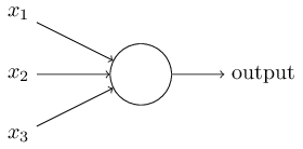
The neuron’s output, 0 or 1, is determined by whether the weighted sum ∑jwjxj is less than or greater than some threshold value:

output=⎧⎩⎨⎪⎪⎪⎪01if ∑jwjxj≤ thresholdif ∑jwjxj> threshold(1)

Let dot product w⋅x≡∑jwjxj, and move the threshold to the other side of the inequality, and to replace it by what’s known as the perceptron’s bias, b≡−threshold, the perceptron rule can be rewritten:

output={01if w⋅x+b≤0if w⋅x+b>0(2)

Perceptrons can be used to compute elementary logical functions such as AND, OR, NAND. In fact, we can use networks of perceptrons to compute any logical function at all. The reason is that the NAND gate is universal for computation, that is, we can build any computation up out of NAND gates.

Sigmoid neurons

To make learning possible, we’d like for a small change in weight to cause only a small corresponding change in the output from the network. If it were true that a small change in a weight (or bias) causes only a small change in output, then we could use this fact to modify the weights and biases to get our network to behave more in the manner we want. A small change in the weights or bias of any single perceptron in the network can sometimes cause the output of that perceptron to completely flip, say from 0 to 1. So it’s not obvious how we can get a network of perceptrons to learn. We can overcome this problem by introducing a new type of artificial neuron called a sigmoid neuron. Sigmoid neurons are similar to perceptrons, but modified so that small changes in their weights and bias cause only a small change in their output. That’s the crucial fact which will allow a network of sigmoid neurons to learn.
We’ll depict sigmoid neurons in the same way we depicted perceptrons. Just like a perceptron, the sigmoid neuron has inputs, x1,x2,…. But instead of being just 0 or 1, these inputs can also take on any values between 0 and 1. Also just like a perceptron, the sigmoid neuron has weights for each input, w1,w2,…, and an overall bias, b. But the output is not 0 or 1. Instead, it’s σ(w⋅x+b), where σ is called the sigmoid function, and is defined by:

σ(z)≡11+e−z.(3)

Incidentally, σ is sometimes called the logistic function, and this new class of neurons called logistic neurons. It’s useful to remember this terminology, since these terms are used by many people working with neural nets. However, we’ll stick with the sigmoid terminology.
To put it all a little more explicitly, the output of a sigmoid neuron with inputs x1,x2,…, weights w1,w2,…, and bias b is:

11+exp(−∑jwjxj−b).(4)

There are many similarities between perceptrons and sigmoid neurons. When z≡w⋅x+b is large and positive, the output from the sigmoid neuron is approximately 1, just as it would have been for a perceptron. When z≡w⋅x+b is very negative, the output from the sigmoid neuron is approximately 0, just as it would have been for a perceptron.
What about the algebraic form of σ? How can we understand that? In fact, the exact form of σ isn’t so important - what really matters is the shape of the function when plotted. Here’s the shape:

By using the actual σ function we get, as already implied above, a smoothed out perceptron. Indeed, it’s the smoothness of the σσ function that is the crucial fact, not its detailed form. The smoothness of σσ means that small changes Δwj in the weights and Δb in the bias will produce a small change Δoutput in the output from the neuron. In fact, calculus tells us that Δoutput is well approximated by:

Δoutput≈∑j∂output∂wjΔwj+∂output∂bΔb,(5)

Δoutput is a linear function of the changes Δwj and Δb in the weights and bias.

The architecture of neural networks

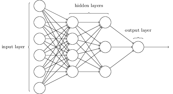
The leftmost layer in this network is called the input layer, and the neurons within the layer are called input neurons. The rightmost or output layer contains the output neurons, or, as in this case, a single output neuron. The middle layer is called a hidden layer, since the neurons in this layer are neither inputs nor outputs. Somewhat confusingly, and for historical reasons, such multiple layer networks are sometimes called multilayer perceptrons or MLPs, despite being made up of sigmoid neurons, not perceptrons.
While the design of the input and output layers of a neural network is often straightforward, there can be quite an art to the design of the hidden layers. In particular, it’s not possible to sum up the design process for the hidden layers with a few simple rules of thumb. Instead, neural networks researchers have developed many design heuristics for the hidden layers, which help people get the behaviour they want out of their nets. For example, such heuristics can be used to help determine how to trade off the number of hidden layers against the time required to train the network.
Up to now, we’ve been discussing neural networks where the output from one layer is used as input to the next layer. Such networks are called feedforward neural networks. This means there are no loops in the network - information is always fed forward, never fed back. There are other models of artificial neural networks in which feedback loops are possible. These models are called recurrent neural networks. The idea in these models is to have neurons which fire for some limited duration of time, before becoming quiescent. That firing can stimulate other neurons, which may fire a little while later, also for a limited duration. That causes still more neurons to fire, and so over time we get a cascade of neurons firing. Loops don’t cause problems in such a model, since a neuron’s output only affects its input at some later time, not instantaneously.

A simple network to classify handwritten digits

To recognize individual digits we will use a three-layer neural network: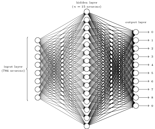
The input layer of the network contains neurons encoding the values of the input pixels. As discussed in the next section, our training data for the network will consist of many 28 by 28 pixel images of scanned handwritten digits, and so the input layer contains 784=28×28 neurons. The input pixels are greyscale, with a value of 0.00.0 representing white, a value of 1.01.0 representing black, and in between values representing gradually darkening shades of grey.
The second layer of the network is a hidden layer. We denote the number of neurons in this hidden layer by n, and we’ll experiment with different values for n.
The output layer of the network contains 10 neurons. A little more precisely, we number the output neurons from 00 through 99, and figure out which neuron has the highest activation value. If that neuron is, say, neuron number 6, then our network will guess that the input digit was a 6. And so on for the other output neurons.

Learning with gradient descent

We’ll use the MNIST data set, which contains tens of thousands of scanned images of handwritten digits, together with their correct classifications. The MNIST data comes in two parts. The first part contains 60,000 images to be used as training data. The images are greyscale and 28 by 28 pixels in size. The second part of the MNIST data set is 10,000 images to be used as test data. Again, these are 28 by 28 greyscale images. We’ll use the test data to evaluate how well our neural network has learned to recognize digits.
We’ll use the notation x to denote a training input. It’ll be convenient to regard each training input x as a 28×28=784-dimensional vector. Each entry in the vector represents the grey value for a single pixel in the image. We’ll denote the corresponding desired output by y=y(x), where y is a 10-dimensional vector. For example, if a particular training image, x, depicts a 6, then y(x)=(0,0,0,0,0,0,1,0,0,0)T is the desired output from the network.
What we’d like is an algorithm which lets us find weights and biases so that the output from the network approximates y(x) for all training inputs x. To quantify how well we’re achieving this goal we define a cost function:

C(w,b)≡12n∑x∥y(x)−a∥2.(6)

Here, w denotes the collection of all weights in the network, b all the biases, n is the total number of training inputs, a is the vector of outputs from the network when x is input, and the sum is over all training inputs, x. Of course, the output aa depends on x, w and b, but to keep the notation simple I haven’t explicitly indicated this dependence. The notation ‖v‖ just denotes the usual length function for a vector v. We’ll call C the quadratic cost function; it’s also sometimes known as the mean squared error or just MSE. So the aim of our training algorithm will be to minimize the cost C(w,b) as a function of the weights and biases. In other words, we want to find a set of weights and biases which make the cost as small as possible. We’ll do that using an algorithm known as gradient descent. Recapping, our goal in training a neural network is to find weights and biases which minimize the quadratic cost function C(w,b).
One way of attacking the problem is to use calculus to try to find the minimum analytically. We could compute derivatives and then try using them to find places where C is an extremum. With some luck that might work when C is a function of just one or a few variables. But it’ll turn into a nightmare when we have many more variables. And for neural networks we’ll often want far more variables - the biggest neural networks have cost functions which depend on billions of weights and biases in an extremely complicated way. Using calculus to minimize that just won’t work!
Suppose in particular that C is a function of m variables, v1,…,vm. Then the change ΔC in C produced by a small change Δv=(Δv1,…,Δvm)T is

ΔC≈∇C⋅Δv,(7)

where the gradient ∇C is the vector

∇C≡(∂C∂v1,…,∂C∂vm)T.(8)

We can choose

Δv=−η∇C,(9)

and we’re guaranteed that our (approximate) expression (7) for ΔC will be negative. This gives us a way of following the gradient to a minimum, even when C is a function of many variables, by repeatedly applying the update rule

v→v′=v−η∇C.(10)

You can think of this update rule as defining the gradient descent algorithm. It gives us a way of repeatedly changing the position v in order to find a minimum of the function C.
Indeed, there’s even a sense in which gradient descent is the optimal strategy for searching for a minimum. Let’s suppose that we’re trying to make a move Δv in position so as to decrease C as much as possible. This is equivalent to minimizing ΔC≈∇C⋅Δv. We’ll constrain the size of the move so that ‖Δv‖=ϵ for some small fixed ϵ>0. In other words, we want a move that is a small step of a fixed size, and we’re trying to find the movement direction which decreases C as much as possible. It can be proved that the choice of Δv which minimizes ∇C⋅Δv is Δv=−η∇C, where η=ϵ/‖∇C‖ is determined by the size constraint ‖Δv‖=ϵ. So gradient descent can be viewed as a way of taking small steps in the direction which does the most to immediately decrease C.
How can we apply gradient descent to learn in a neural network? The idea is to use gradient descent to find the weights wk and biases bl which minimize the cost in Equation (6). To see how this works, let’s restate the gradient descent update rule, with the weights and biases replacing the variables vj. In other words, our “position” now has components wk and bl, and the gradient vector ∇C has corresponding components ∂C/∂wk and ∂C/∂bl. Writing out the gradient descent update rule in terms of components, we have

wkbl→→w′k=wk−η∂C∂wkb′l=bl−η∂C∂bl.(11)(12)

By repeatedly applying this update rule we can “roll down the hill”, and hopefully find a minimum of the cost function. In other words, this is a rule which can be used to learn in a neural network.
Notice that this cost function has the form C=1n∑xCx, that is, it’s an average over costs Cx≡‖y(x)−a‖/2 for individual training examples. In practice, to compute the gradient ∇C we need to compute the gradients ∇Cx separately for each training input, x, and then average them, ∇C=1n∑x∇Cx. Unfortunately, when the number of training inputs is very large this can take a long time, and learning thus occurs slowly.
An idea called stochastic gradient descent can be used to speed up learning. The idea is to estimate the gradient ∇C by computing ∇Cx for a small sample of randomly chosen training inputs. By averaging over this small sample it turns out that we can quickly get a good estimate of the true gradient ∇C, and this helps speed up gradient descent, and thus learning.
To make these ideas more precise, stochastic gradient descent works by randomly picking out a small number mm of randomly chosen training inputs. We’ll label those random training inputs X1,X2,…,Xm, and refer to them as a mini-batch. Provided the sample size mm is large enough we expect that the average value of the ∇CXj will be roughly equal to the average over all ∇Cx, that is,

∑mj=1∇CXjm≈∑x∇Cxn=∇C,(13)

confirming that we can estimate the overall gradient by computing gradients just for the randomly chosen mini-batch.
To connect this explicitly to learning in neural networks, suppose wk and bl denote the weights and biases in our neural network. Then stochastic gradient descent works by picking out a randomly chosen mini-batch of training inputs, and training with those,

wkbl→→w′k=wk−ηm∑j∂CXj∂wkb′l=bl−ηm∑j∂CXj∂bl,(14)(15)

where the sums are over all the training examples Xj in the current mini-batch. Then we pick out another randomly chosen mini-batch and train with those. And so on, until we’ve exhausted the training inputs, which is said to complete an epoch of training. At that point we start over with a new training epoch.
If we have a training set of size n=60,000, as in MNIST, and choose a mini-batch size of (say) m=10, this means we’ll get a factor of 6,000 speedup in estimating the gradient! Of course, the estimate won’t be perfect - there will be statistical fluctuations - but it doesn’t need to be perfect: all we really care about is moving in a general direction that will help decrease C, and that means we don’t need an exact computation of the gradient. In practice, stochastic gradient descent is a commonly used and powerful technique for learning in neural networks.

Implementing our network to classify digits

git clone https://github.com/mnielsen/neural-networks-and-deep-learning.git

Incidentally, when I described the MNIST data earlier, I said it was split into 60,000 training images, and 10,000 test images. That’s the official MNIST description. Actually, we’re going to split the data a little differently. We’ll leave the test images as is, but split the 60,000-image MNIST training set into two parts: a set of 50,000 images, which we’ll use to train our neural network, and a separate 10,000 image validation set. We won’t use the validation data in this chapter, but later in the book we’ll find it useful in figuring out how to set certain hyper-parameters of the neural network - things like the learning rate, and so on, which aren’t directly selected by our learning algorithm. Although the validation data isn’t part of the original MNIST specification, many people use MNIST in this fashion, and the use of validation data is common in neural networks. When I refer to the “MNIST training data” from now on, I’ll be referring to our 50,000 image data set, not the original 60,000 image data set.
The centerpiece is a Network class, which we use to represent a neural network. Here’s the code we use to initialize a Network object:

class Network(object):    def __init__(self, sizes):        self.num_layers = len(sizes)        self.sizes = sizes        self.biases = [np.random.randn(y, 1) for y in sizes[1:]]        self.weights = [np.random.randn(y, x)                         for x, y in zip(sizes[:-1], sizes[1:])]

In this code, the list sizes contains the number of neurons in the respective layers. So, for example, if we want to create a Network object with 2 neurons in the first layer, 3 neurons in the second layer, and 1 neuron in the final layer, we’d do this with the code:

net = Network([2, 3, 1])

The biases and weights in the Network object are all initialized randomly, using the Numpy np.random.randn function to generate Gaussian distributions with mean 0 and standard deviation 1. This random initialization gives our stochastic gradient descent algorithm a place to start from. In later chapters we’ll find better ways of initializing the weights and biases, but this will do for now. Note that the Network initialization code assumes that the first layer of neurons is an input layer, and omits to set any biases for those neurons, since biases are only ever used in computing the outputs from later layers.
Note also that the biases and weights are stored as lists of Numpy matrices. So, for example net.weights[1] is a Numpy matrix storing the weights connecting the second and third layers of neurons. (It’s not the first and second layers, since Python’s list indexing starts at 0.) Since net.weights[1] is rather verbose, let’s just denote that matrix w. It’s a matrix such that wjk is the weight for the connection between the kth neuron in the second layer, and the jth neuron in the third layer. This ordering of the j and k indices may seem strange - surely it’d make more sense to swap the j and k indices around? The big advantage of using this ordering is that it means that the vector of activations of the third layer of neurons is:

a′=σ(wa+b).(16)

There’s quite a bit going on in this equation, so let’s unpack it piece by piece. aa is the vector of activations of the second layer of neurons. To obtain a′ we multiply a by the weight matrix w, and add the vector b of biases. We then apply the function σ elementwise to every entry in the vector wa+b. It’s easy to verify that Equation (16) gives the same result as our earlier rule, Equation (4), for computing the output of a sigmoid neuron.

def sigmoid(z):    return 1.0/(1.0+np.exp(-z))

We then add a feedforward method to the Network class, which, given an input a for the network, returns the corresponding output. All the method does is applies Equation (16) for each layer:

    def feedforward(self, a):        """Return the output of the network if "a" is input."""        for b, w in zip(self.biases, self.weights):            a = sigmoid(np.dot(w, a)+b)        return a

Of course, the main thing we want our Network objects to do is to learn. To that end we’ll give them an SGD method which implements stochastic gradient descent. Here’s the code. It’s a little mysterious in a few places, but I’ll break it down below, after the listing.

    def SGD(self, training_data, epochs, mini_batch_size, eta,            test_data=None):        """Train the neural network using mini-batch stochastic        gradient descent.  The "training_data" is a list of tuples        "(x, y)" representing the training inputs and the desired        outputs.  The other non-optional parameters are        self-explanatory.  If "test_data" is provided then the        network will be evaluated against the test data after each        epoch, and partial progress printed out.  This is useful for        tracking progress, but slows things down substantially."""        if test_data: n_test = len(test_data)        n = len(training_data)        for j in xrange(epochs):            random.shuffle(training_data)            mini_batches = [                training_data[k:k+mini_batch_size]                for k in xrange(0, n, mini_batch_size)]            for mini_batch in mini_batches:                self.update_mini_batch(mini_batch, eta)            if test_data:                print "Epoch {0}: {1} / {2}".format(                    j, self.evaluate(test_data), n_test)            else:                print "Epoch {0} complete".format(j)

The training_data is a list of tuples (x, y) representing the training inputs and corresponding desired outputs. The variables epochs and mini_batch_size are what you’d expect - the number of epochs to train for, and the size of the mini-batches to use when sampling. eta is the learning rate, η. If the optional argument test_data is supplied, then the program will evaluate the network after each epoch of training, and print out partial progress. This is useful for tracking progress, but slows things down substantially.
The code works as follows. In each epoch, it starts by randomly shuffling the training data, and then partitions it into mini-batches of the appropriate size. This is an easy way of sampling randomly from the training data. Then for each mini_batch we apply a single step of gradient descent. This is done by the code self.update_mini_batch(mini_batch, eta), which updates the network weights and biases according to a single iteration of gradient descent, using just the training data in mini_batch. Here’s the code for the update_mini_batch method:

    def update_mini_batch(self, mini_batch, eta):        """Update the network's weights and biases by applying        gradient descent using backpropagation to a single mini batch.        The "mini_batch" is a list of tuples "(x, y)", and "eta"        is the learning rate."""        nabla_b = [np.zeros(b.shape) for b in self.biases]        nabla_w = [np.zeros(w.shape) for w in self.weights]        for x, y in mini_batch:            delta_nabla_b, delta_nabla_w = self.backprop(x, y)            nabla_b = [nb+dnb for nb, dnb in zip(nabla_b, delta_nabla_b)]            nabla_w = [nw+dnw for nw, dnw in zip(nabla_w, delta_nabla_w)]        self.weights = [w-(eta/len(mini_batch))*nw                         for w, nw in zip(self.weights, nabla_w)]        self.biases = [b-(eta/len(mini_batch))*nb                        for b, nb in zip(self.biases, nabla_b)]

Most of the work is done by the line

            delta_nabla_b, delta_nabla_w = self.backprop(x, y)

This invokes something called the backpropagation algorithm, which is a fast way of computing the gradient of the cost function. So update_mini_batch works simply by computing these gradients for every training example in the mini_batch, and then updating self.weights and self.biases appropriately.

I’m not going to show the code for self.backprop right now. We’ll study how backpropagation works in the next chapter, including the code for self.backprop. For now, just assume that it behaves as claimed, returning the appropriate gradient for the cost associated to the training example x.

"""network.py~~~~~~~~~~A module to implement the stochastic gradient descent learningalgorithm for a feedforward neural network.  Gradients are calculatedusing backpropagation.  Note that I have focused on making the codesimple, easily readable, and easily modifiable.  It is not optimized,and omits many desirable features."""#### Libraries# Standard libraryimport random# Third-party librariesimport numpy as npclass Network(object):    def __init__(self, sizes):        """The list ``sizes`` contains the number of neurons in the        respective layers of the network.  For example, if the list        was [2, 3, 1] then it would be a three-layer network, with the        first layer containing 2 neurons, the second layer 3 neurons,        and the third layer 1 neuron.  The biases and weights for the        network are initialized randomly, using a Gaussian        distribution with mean 0, and variance 1.  Note that the first        layer is assumed to be an input layer, and by convention we        won't set any biases for those neurons, since biases are only        ever used in computing the outputs from later layers."""        self.num_layers = len(sizes)        self.sizes = sizes        self.biases = [np.random.randn(y, 1) for y in sizes[1:]]        self.weights = [np.random.randn(y, x)                        for x, y in zip(sizes[:-1], sizes[1:])]    def feedforward(self, a):        """Return the output of the network if ``a`` is input."""        for b, w in zip(self.biases, self.weights):            a = sigmoid(np.dot(w, a)+b)        return a    def SGD(self, training_data, epochs, mini_batch_size, eta,            test_data=None):        """Train the neural network using mini-batch stochastic        gradient descent.  The ``training_data`` is a list of tuples        ``(x, y)`` representing the training inputs and the desired        outputs.  The other non-optional parameters are        self-explanatory.  If ``test_data`` is provided then the        network will be evaluated against the test data after each        epoch, and partial progress printed out.  This is useful for        tracking progress, but slows things down substantially."""        if test_data: n_test = len(test_data)        n = len(training_data)        for j in xrange(epochs):            random.shuffle(training_data)            mini_batches = [                training_data[k:k+mini_batch_size]                for k in xrange(0, n, mini_batch_size)]            for mini_batch in mini_batches:                self.update_mini_batch(mini_batch, eta)            if test_data:                print "Epoch {0}: {1} / {2}".format(                    j, self.evaluate(test_data), n_test)            else:                print "Epoch {0} complete".format(j)    def update_mini_batch(self, mini_batch, eta):        """Update the network's weights and biases by applying        gradient descent using backpropagation to a single mini batch.        The ``mini_batch`` is a list of tuples ``(x, y)``, and ``eta``        is the learning rate."""        nabla_b = [np.zeros(b.shape) for b in self.biases]        nabla_w = [np.zeros(w.shape) for w in self.weights]        for x, y in mini_batch:            delta_nabla_b, delta_nabla_w = self.backprop(x, y)            nabla_b = [nb+dnb for nb, dnb in zip(nabla_b, delta_nabla_b)]            nabla_w = [nw+dnw for nw, dnw in zip(nabla_w, delta_nabla_w)]        self.weights = [w-(eta/len(mini_batch))*nw                        for w, nw in zip(self.weights, nabla_w)]        self.biases = [b-(eta/len(mini_batch))*nb                       for b, nb in zip(self.biases, nabla_b)]    def backprop(self, x, y):        """Return a tuple ``(nabla_b, nabla_w)`` representing the        gradient for the cost function C_x.  ``nabla_b`` and        ``nabla_w`` are layer-by-layer lists of numpy arrays, similar        to ``self.biases`` and ``self.weights``."""        nabla_b = [np.zeros(b.shape) for b in self.biases]        nabla_w = [np.zeros(w.shape) for w in self.weights]        # feedforward        activation = x        activations = [x] # list to store all the activations, layer by layer        zs = [] # list to store all the z vectors, layer by layer        for b, w in zip(self.biases, self.weights):            z = np.dot(w, activation)+b            zs.append(z)            activation = sigmoid(z)            activations.append(activation)        # backward pass        delta = self.cost_derivative(activations[-1], y) * \            sigmoid_prime(zs[-1])        nabla_b[-1] = delta        nabla_w[-1] = np.dot(delta, activations[-2].transpose())        # Note that the variable l in the loop below is used a little        # differently to the notation in Chapter 2 of the book.  Here,        # l = 1 means the last layer of neurons, l = 2 is the        # second-last layer, and so on.  It's a renumbering of the        # scheme in the book, used here to take advantage of the fact        # that Python can use negative indices in lists.        for l in xrange(2, self.num_layers):            z = zs[-l]            sp = sigmoid_prime(z)            delta = np.dot(self.weights[-l+1].transpose(), delta) * sp            nabla_b[-l] = delta            nabla_w[-l] = np.dot(delta, activations[-l-1].transpose())        return (nabla_b, nabla_w)    def evaluate(self, test_data):        """Return the number of test inputs for which the neural        network outputs the correct result. Note that the neural        network's output is assumed to be the index of whichever        neuron in the final layer has the highest activation."""        test_results = [(np.argmax(self.feedforward(x)), y)                        for (x, y) in test_data]        return sum(int(x == y) for (x, y) in test_results)    def cost_derivative(self, output_activations, y):        """Return the vector of partial derivatives \partial C_x /        \partial a for the output activations."""        return (output_activations-y)#### Miscellaneous functionsdef sigmoid(z):    """The sigmoid function."""    return 1.0/(1.0+np.exp(-z))def sigmoid_prime(z):    """Derivative of the sigmoid function."""    return sigmoid(z)*(1-sigmoid(z))

How well does the program recognize handwritten digits? Well, let’s start by loading in the MNIST data. I’ll do this using a little helper program, mnist_loader.py, to be described below. We execute the following commands in a Python shell,

>>> import mnist_loader>>> training_data, validation_data, test_data = \... mnist_loader.load_data_wrapper()

After loading the MNIST data, we’ll set up a Network with 3030 hidden neurons. We do this after importing the Python program listed above, which is named network,

>>> import network>>> net = network.Network([784, 30, 10])

Finally, we’ll use stochastic gradient descent to learn from the MNIST training_data over 30 epochs, with a mini-batch size of 10, and a learning rate of η=3.0,

>>> net.SGD(training_data, 30, 10, 3.0, test_data=test_data)

here is a partial transcript of the output of one training run of the neural network. The transcript shows the number of test images correctly recognized by the neural network after each epoch of training. As you can see, after just a single epoch this has reached 9,129 out of 10,000, and the number continues to grow,

Epoch 0: 9129 / 10000Epoch 1: 9295 / 10000Epoch 2: 9348 / 10000...Epoch 27: 9528 / 10000Epoch 28: 9542 / 10000Epoch 29: 9534 / 10000

That is, the trained network gives us a classification rate of about 9595 percent - 95.4295.42 percent at its peak (“Epoch 28”)!

Toward deep learning

The end result is a network which breaks down a very complicated question - does this image show a face or not - into very simple questions answerable at the level of single pixels. It does this through a series of many layers, with early layers answering very simple and specific questions about the input image, and later layers building up a hierarchy of ever more complex and abstract concepts. Networks with this kind of many-layer structure - two or more hidden layers - are called deep neural networks.
Of course, I haven’t said how to do this recursive decomposition into sub-networks. It certainly isn’t practical to hand-design the weights and biases in the network. Instead, we’d like to use learning algorithms so that the network can automatically learn the weights and biases - and thus, the hierarchy of concepts - from training data. Researchers in the 1980s and 1990s tried using stochastic gradient descent and backpropagation to train deep networks. Unfortunately, except for a few special architectures, they didn’t have much luck. The networks would learn, but very slowly, and in practice often too slowly to be useful.
Since 2006, a set of techniques has been developed that enable learning in deep neural nets. These deep learning techniques are based on stochastic gradient descent and backpropagation, but also introduce new ideas. These techniques have enabled much deeper (and larger) networks to be trained - people now routinely train networks with 5 to 10 hidden layers. And, it turns out that these perform far better on many problems than shallow neural networks, i.e., networks with just a single hidden layer. The reason, of course, is the ability of deep nets to build up a complex hierarchy of concepts.