spark厦大----逻辑斯蒂回归分类器--spark.ml

来源：http://mocom.xmu.edu.cn/article/show/586679ecaa2c3f280956e7af/0/1

方法简介

​ 逻辑斯蒂回归（logistic regression）是统计学习中的经典分类方法，属于对数线性模型。logistic回归的因变量可以是二分类的，也可以是多分类的。

基本原理

logistic分布

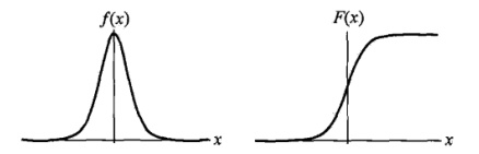
​ 设X是连续随机变量，X服从logistic分布是指X具有下列分布函数和密度函数：

​ $$F\left(x\right)=P(x\le x)=\frac{1}{1+e^{-(x-\mu )/\gamma }}$$

​ $$f\left(x\right)=F^{{}^{\prime }}\left(x\right)=\frac{e^{-(x-\mu )/\gamma }}{\gamma (1+e^{-(x-\mu )/\gamma }{)}^2}$$

​ 其中，$\mu$为位置参数，$\gamma$为形状参数。

​ $f\left(x\right)$与$F\left(x\right)$图像如下，其中分布函数是以$(\mu ,\frac{1}{2})$为中心对阵，$\gamma$越小曲线变化越快。

二项logistic回归模型：

​ 二项logistic回归模型如下：

​ $$P(Y=1|x)=\frac{exp(w\cdot x+b)}{1+exp(w\cdot x+b)}$$

​ $$P(Y=0|x)=\frac{1}{1+exp(w\cdot x+b)}$$

​ 其中，$x\in R^n$是输入，$Y\in 0,1$是输出，w称为权值向量，b称为偏置，$w\cdot x$为w和x的内积。

参数估计

​ 假设：

​ $$P(Y=1|x)=\pi \left(x\right),P(Y=0|x)=1-\pi \left(x\right)$$

​ 则采用“极大似然法”来估计w和b。似然函数为:

​ $$\prod _{i=1}^N\left[\pi \right(x_i\left){]}^{y_i}\right[1-\pi \left(x_i\right){]}^{1-y_i}$$

​ 为方便求解，对其“对数似然”进行估计：

​ $$L\left(w\right)=\sum _{i=1}^N[y_i\log \pi \left(x_i\right)+(1-y_i\left)\log (1-\pi (x_i)\right)]$$

​ 从而对$L\left(w\right)$求极大值，得到$w$的估计值。求极值的方法可以是梯度下降法，梯度上升法等。

示例代码

​ 我们以iris数据集（https://archive.ics.uci.edu/ml/machine-learning-databases/iris/iris.data）为例进行分析。iris以鸢尾花的特征作为数据来源，数据集包含150个数据集，分为3类，每类50个数据，每个数据包含4个属性，是在数据挖掘、数据分类中非常常用的测试集、训练集。为了便于理解，这里主要用后两个属性（花瓣的长度和宽度）来进行分类。由于目前spark.ml 中只支持二分类，此处取其中的后两类数据进行分析。

1. 导入需要的包：

import org.apache.spark.SparkConfimport org.apache.spark.SparkContextimport org.apache.spark.sql.SQLContextimport org.apache.spark.ml.{Pipeline,PipelineModel}import org.apache.spark.ml.classification.LogisticRegressionimport org.apache.spark.ml.evaluation.MulticlassClassificationEvaluatorimport org.apache.spark.ml.feature.{IndexToString, StringIndexer, VectorIndexer,HashingTF, Tokenizer}import org.apache.spark.mllib.linalg.{Vector,Vectors}import org.apache.spark.sql.Rowimport org.apache.spark.mllib.stat.{MultivariateStatisticalSummary, Statistics}import org.apache.spark.ml.classification.LogisticRegressionModel

2. 读取数据，简要分析：

​ 首先根据SparkContext来创建一个SQLContext，其中sc是一个已经存在的SparkContext；然后导入sqlContext.implicits._来实现RDD到Dataframe的隐式转换。

scala> val sqlContext = new SQLContext(sc)sqlContext: org.apache.spark.sql.SQLContext = org.apache.spark.sql.SQLContext@10d83860scala> import sqlContext.implicits._import sqlContext.implicits._

​ 读取文本文件，第一个map把每行的数据用“,”隔开。比如数据集中，每行被分成了5部分，前4部分是鸢尾花的4个特征，最后一部分是鸢尾花的分类；前面说到，我们这里主要用后两个属性（花瓣的长度和宽度）来进行分类，所以在下一个map中我们获取到这两个属性，存储在Vector中。

scala> val observations=sc.textFile("G:/spark/iris.data").map(_.split(",")).map(p => Vectors.dense(p(2).toDouble, p(3).toDouble))observations: org.apache.spark.rdd.RDD[org.apache.spark.mllib.linalg.Vector] = MapPartitionsRDD[14] at map at :37

​ 接下来，调用mllib.stat中的统计方法得到数据的基本的统计信息，例如均值、方差等。colStats() 方法返回一个MultivariateStatisticalSummary的实例，其中包含每列的最大值、最小值、均值等等。这里简单的列出了一些基本的统计结果。

scala> val summary: MultivariateStatisticalSummary = Statistics.colStats(observations)summary: org.apache.spark.mllib.stat.MultivariateStatisticalSummary = org.apache.spark.mllib.stat.MultivariateOnlineSummarizer@1a5462adscala> println(summary.mean)[3.7586666666666666,1.1986666666666668]scala> println(summary.variance)[3.113179418344516,0.5824143176733783]scala> println(summary.numNonzeros)[150.0,150.0]

​ 用case class定义一个schema:Iris，Iris就是需要的数据的结构；然后读取数据，创建一个Iris模式的RDD，然后转化成dataframe；最后调用show()方法来查看一下部分数据。

scala> case class Iris(features: Vector, label: String)defined class Irisscala> val data = sc.textFile("G:/spark/iris.data")          |       .map(_.split(","))          |       .map(p => Iris(Vectors.dense(p(2).toDouble, p(3).toDouble), p(4).toString()))          |       .toDF()data: org.apache.spark.sql.DataFrame = [features: vector, label: string]scala> data.show()+---------+-----------+| features|      label|+---------+-----------+|[1.4,0.2]|Iris-setosa||[1.4,0.2]|Iris-setosa||[1.3,0.2]|Iris-setosa||[1.5,0.2]|Iris-setosa||[1.4,0.2]|Iris-setosa||[1.7,0.4]|Iris-setosa||[1.4,0.3]|Iris-setosa||[1.5,0.2]|Iris-setosa||[1.4,0.2]|Iris-setosa||[1.5,0.1]|Iris-setosa||[1.5,0.2]|Iris-setosa||[1.6,0.2]|Iris-setosa||[1.4,0.1]|Iris-setosa||[1.1,0.1]|Iris-setosa||[1.2,0.2]|Iris-setosa||[1.5,0.4]|Iris-setosa||[1.3,0.4]|Iris-setosa||[1.4,0.3]|Iris-setosa||[1.7,0.3]|Iris-setosa||[1.5,0.3]|Iris-setosa|+---------+-----------+only showing top 20 rows

​ 有的时候不需要全部的数据，比如ml库中的logistic回归目前只支持2分类，所以要从中选出两类的数据。这里首先把刚刚得到的数据注册成一个表iris，注册成这个表之后，就可以通过sql语句进行数据查询，比如这里选出了所有不属于“Iris-setosa”类别的数据。选出需要的数据后，把结果打印出来看一下，这时就已经没有“Iris-setosa”类别的数据。

scala> data.registerTempTable("iris")scala> val df = sqlContext.sql("select * from iris where label != 'Iris-setosa'")df: org.apache.spark.sql.DataFrame = [features: vector, label: string]scala>     df.map(t => t(1)+":"+t(0)).collect().foreach(println)Iris-versicolor:[4.7,1.4]Iris-versicolor:[4.5,1.5]Iris-versicolor:[4.9,1.5]Iris-versicolor:[4.0,1.3]Iris-versicolor:[4.6,1.5]Iris-versicolor:[4.5,1.3]... ...

3. 构建ML的pipeline

​ 分别获取标签列和特征列，进行索引，并进行了重命名。

scala> val labelIndexer = new StringIndexer().setInputCol("label").setOutputCol("indexedLabel").fit(df)labelIndexer: org.apache.spark.ml.feature.StringIndexerModel = strIdx_a14ddbf05040scala> val featureIndexer = new VectorIndexer().setInputCol("features").setOutputCol("indexedFeatures").fit(df)featureIndexer: org.apache.spark.ml.feature.VectorIndexerModel = vecIdx_755d3f41691a

​ 接下来，把数据集随机分成训练集和测试集，其中训练集占70%。

scala> val Array(trainingData, testData) = df.randomSplit(Array(0.7, 0.3))trainingData: org.apache.spark.sql.DataFrame = [features: vector, label: string]testData: org.apache.spark.sql.DataFrame = [features: vector, label: string]

​ 然后，设置logistic的参数，这里我们统一用setter的方法来设置，也可以用ParamMap来设置（具体的可以查看spark mllib的官网）。这里设置了循环次数为10次，正则化项为0.3等，具体的可以设置的参数可以通过explainParams()来获取，还能看到程序已经设置的参数的结果。

scala>     val lr = new LogisticRegression().     |       setLabelCol("indexedLabel").     |       setFeaturesCol("indexedFeatures").     |       setMaxIter(10).     |       setRegParam(0.3).     |       setElasticNetParam(0.8)lr: org.apache.spark.ml.classification.LogisticRegression = logreg_a58ee56c357fscala> println("LogisticRegression parameters:\n" + lr.explainParams() + "\n")LogisticRegression parameters:elasticNetParam: the ElasticNet mixing parameter, in range [0, 1]. For alpha = 0, the penalty is an L2 penalty. For alpha = 1, it is an L1 penalty (default: 0.0, current: 0.8)featuresCol: features column name (default: features, current: indexedFeatures)fitIntercept: whether to fit an intercept term (default: true)labelCol: label column name (default: label, current: indexedLabel)maxIter: maximum number of iterations (>= 0) (default: 100, current: 10)predictionCol: prediction column name (default: prediction)probabilityCol: Column name for predicted class conditional probabilities. Note: Not all models output well-calibrated probability estimates! These probabilities should be treated as confidences, not precise probabilities (default: probability)rawPredictionCol: raw prediction (a.k.a. confidence) column name (default: rawPrediction)regParam: regularization parameter (>= 0) (default: 0.0, current: 0.3)standardization: whether to standardize the training features before fitting the model (default: true)threshold: threshold in binary classification prediction, in range [0, 1] (default: 0.5)thresholds: Thresholds in multi-class classification to adjust the probability of predicting each class. Array must have length equal to the number of classes, with values >= 0. The class with largest value p/t is predicted, where p is the original probability of that class and t is the class' threshold. (undefined)tol: the convergence tolerance for iterative algorithms (default: 1.0E-6)weightCol: weight column name. If this is not set or empty, we treat all instance weights as 1.0. (default: )

​ 这里设置一个labelConverter，目的是把预测的类别重新转化成字符型的。

scala>     val labelConverter = new IndexToString().     |       setInputCol("prediction").     |       setOutputCol("predictedLabel").     |       setLabels(labelIndexer.labels)labelConverter: org.apache.spark.ml.feature.IndexToString = idxToStr_89b2b1508b35

​ 构建pipeline，设置stage，然后调用fit()来训练模型。

scala>     val pipeline = new Pipeline().     |       setStages(Array(labelIndexer, featureIndexer, lr, labelConverter))pipeline: org.apache.spark.ml.Pipeline = pipeline_33fa7f88685ascala> val model = pipeline.fit(trainingData)model: org.apache.spark.ml.PipelineModel = pipeline_33fa7f88685a

​ pipeline本质上是一个评估器（Estimator），当pipeline调用fit()的时候就产生了一个PipelineModel，本质上是一个转换器（Transformer）。然后这个PipelineModel就可以调用transform()来进行预测，生成一个新的DataFrame，即利用训练得到的模型对测试集进行验证。

scala> val predictions = model.transform(testData)predictions: org.apache.spark.sql.DataFrame = [features: vector, label: string,indexedLabel: double, indexedFeatures: vector, rawPrediction: vector, probability: vector, prediction: double, predictedLabel: string]

​ 最后输出预测的结果，其中select选择要输出的列，collect获取所有行的数据，用foreach把每行打印出来。

scala> predictions.     |       select("predictedLabel", "label", "features", "probability").     |       collect().     |       foreach { case Row(predictedLabel: String, label: String, features: Vector, prob: Vector) =>     |         println(s"($label, $features) --> prob=$prob, predictedLabel=$predictedLabel")     |     }(Iris-versicolor, [3.5,1.0]) --> prob=[0.6949117083297265,0.30508829167027346], predictedLabel=Iris-versicolor(Iris-versicolor, [4.1,1.0]) --> prob=[0.694606868968713,0.30539313103128685], predictedLabel=Iris-versicolor(Iris-versicolor, [4.3,1.3]) --> prob=[0.6060637422536634,0.3939362577463365], predictedLabel=Iris-versicolor(Iris-versicolor, [4.4,1.4]) --> prob=[0.5745401752760255,0.4254598247239745], predictedLabel=Iris-versicolor(Iris-versicolor, [4.5,1.3]) --> prob=[0.6059493387519529,0.39405066124804705],predictedLabel=Iris-versicolor(Iris-versicolor, [4.5,1.5]) --> prob=[0.5423986730485701,0.45760132695142974],... ...

4. 模型评估

​ 创建一个MulticlassClassificationEvaluator实例，用setter方法把预测分类的列名和真实分类的列名进行设置；然后计算预测准确率和错误率。

scala> val evaluator = new MulticlassClassificationEvaluator().     |       setLabelCol("indexedLabel").     |       setPredictionCol("prediction")evaluator: org.apache.spark.ml.evaluation.MulticlassClassificationEvaluator = mcEval_198b7e595a62scala> val accuracy = evaluator.evaluate(predictions)accuracy: Double = 0.9411764705882353scala> println("Test Error = " + (1.0 - accuracy))Test Error = 0.05882352941176472

​ 从上面可以看到预测的准确性达到94.1%，接下来可以通过model来获取训练得到的逻辑斯蒂模型。前面已经说过model是一个PipelineModel，因此可以通过调用它的stages来获取模型，具体如下：

scala> val lrModel = model.stages(2).asInstanceOf[LogisticRegressionModel]lrModel: org.apache.spark.ml.classification.LogisticRegressionModel = logreg_a58ee56c357fscala> println("Coefficients: " + lrModel.coefficients+"Intercept: "+lrModel.intercept+     |         "numClasses: "+lrModel.numClasses+"numFeatures: "+lrModel.numFeatures)Coefficients: [0.0023957582955816056,0.13015697498232498]Intercept: -0.8315687375527291numClasses: 2numFeatures: 2