python + sklearn ︱分类效果评估——acc、recall、F1、ROC、回归、距离

之前提到过聚类之后，聚类质量的评价：
聚类︱python实现 六大 分群质量评估指标（兰德系数、互信息、轮廓系数）
R语言相关分类效果评估：
R语言︱分类器的性能表现评价（混淆矩阵，准确率，召回率，F1,mAP、ROC曲线）

.

---

一、acc、recall、F1、混淆矩阵、分类综合报告

1、准确率

第一种方式：accuracy_score

# 准确率import numpy as npfrom sklearn.metrics import accuracy_scorey_pred = [0, 2, 1, 3,9,9,8,5,8]y_true = [0, 1, 2, 3,2,6,3,5,9]accuracy_score(y_true, y_pred)Out[127]: 0.33333333333333331accuracy_score(y_true, y_pred, normalize=False)  # 类似海明距离，每个类别求准确后，再求微平均Out[128]: 3

第二种方式：metrics

宏平均比微平均更合理，但也不是说微平均一无是处，具体使用哪种评测机制，还是要取决于数据集中样本分布

宏平均（Macro-averaging），是先对每一个类统计指标值，然后在对所有类求算术平均值。
微平均（Micro-averaging），是对数据集中的每一个实例不分类别进行统计建立全局混淆矩阵，然后计算相应指标。（来源：谈谈评价指标中的宏平均和微平均）

from sklearn import metricsmetrics.precision_score(y_true, y_pred, average='micro')  # 微平均，精确率Out[130]: 0.33333333333333331metrics.precision_score(y_true, y_pred, average='macro')  # 宏平均，精确率Out[131]: 0.375metrics.precision_score(y_true, y_pred, labels=[0, 1, 2, 3], average='macro')  # 指定特定分类标签的精确率Out[133]: 0.5

其中average参数有五种：(None, ‘micro’, ‘macro’, ‘weighted’, ‘samples’)
.

2、召回率

metrics.recall_score(y_true, y_pred, average='micro')Out[134]: 0.33333333333333331metrics.recall_score(y_true, y_pred, average='macro')Out[135]: 0.3125

.

3、F1

metrics.f1_score(y_true, y_pred, average='weighted')  Out[136]: 0.37037037037037035

.

4、混淆矩阵

# 混淆矩阵from sklearn.metrics import confusion_matrixconfusion_matrix(y_true, y_pred)Out[137]: array([[1, 0, 0, ..., 0, 0, 0],       [0, 0, 1, ..., 0, 0, 0],       [0, 1, 0, ..., 0, 0, 1],       ...,        [0, 0, 0, ..., 0, 0, 1],       [0, 0, 0, ..., 0, 0, 0],       [0, 0, 0, ..., 0, 1, 0]])

横为true label 竖为predict

.

5、 分类报告

# 分类报告：precision/recall/fi-score/均值/分类个数 from sklearn.metrics import classification_report y_true = [0, 1, 2, 2, 0] y_pred = [0, 0, 2, 2, 0] target_names = ['class 0', 'class 1', 'class 2'] print(classification_report(y_true, y_pred, target_names=target_names))

其中的结果：

             precision    recall  f1-score   support    class 0       0.67      1.00      0.80         2    class 1       0.00      0.00      0.00         1    class 2       1.00      1.00      1.00         2avg / total       0.67      0.80      0.72         5

包含：precision/recall/fi-score/均值/分类个数
.

6、 kappa score

kappa score是一个介于(-1, 1)之间的数. score>0.8意味着好的分类；0或更低意味着不好（实际是随机标签）

 from sklearn.metrics import cohen_kappa_score y_true = [2, 0, 2, 2, 0, 1] y_pred = [0, 0, 2, 2, 0, 2] cohen_kappa_score(y_true, y_pred)

.

---

二、ROC

1、计算ROC值

import numpy as np from sklearn.metrics import roc_auc_score y_true = np.array([0, 0, 1, 1]) y_scores = np.array([0.1, 0.4, 0.35, 0.8]) roc_auc_score(y_true, y_scores)

2、ROC曲线

 y = np.array([1, 1, 2, 2]) scores = np.array([0.1, 0.4, 0.35, 0.8]) fpr, tpr, thresholds = roc_curve(y, scores, pos_label=2)

来看一个官网例子，贴部分代码，全部的code见：Receiver Operating Characteristic (ROC)

import numpy as npimport matplotlib.pyplot as pltfrom itertools import cyclefrom sklearn import svm, datasetsfrom sklearn.metrics import roc_curve, aucfrom sklearn.model_selection import train_test_splitfrom sklearn.preprocessing import label_binarizefrom sklearn.multiclass import OneVsRestClassifierfrom scipy import interp# Import some data to play withiris = datasets.load_iris()X = iris.datay = iris.target# 画图all_fpr = np.unique(np.concatenate([fpr[i] for i in range(n_classes)]))# Then interpolate all ROC curves at this pointsmean_tpr = np.zeros_like(all_fpr)for i in range(n_classes):    mean_tpr += interp(all_fpr, fpr[i], tpr[i])# Finally average it and compute AUCmean_tpr /= n_classesfpr["macro"] = all_fprtpr["macro"] = mean_tprroc_auc["macro"] = auc(fpr["macro"], tpr["macro"])# Plot all ROC curvesplt.figure()plt.plot(fpr["micro"], tpr["micro"],         label='micro-average ROC curve (area = {0:0.2f})'               ''.format(roc_auc["micro"]),         color='deeppink', linestyle=':', linewidth=4)plt.plot(fpr["macro"], tpr["macro"],         label='macro-average ROC curve (area = {0:0.2f})'               ''.format(roc_auc["macro"]),         color='navy', linestyle=':', linewidth=4)colors = cycle(['aqua', 'darkorange', 'cornflowerblue'])for i, color in zip(range(n_classes), colors):    plt.plot(fpr[i], tpr[i], color=color, lw=lw,             label='ROC curve of class {0} (area = {1:0.2f})'             ''.format(i, roc_auc[i]))plt.plot([0, 1], [0, 1], 'k--', lw=lw)plt.xlim([0.0, 1.0])plt.ylim([0.0, 1.05])plt.xlabel('False Positive Rate')plt.ylabel('True Positive Rate')plt.title('Some extension of Receiver operating characteristic to multi-class')plt.legend(loc="lower right")plt.show()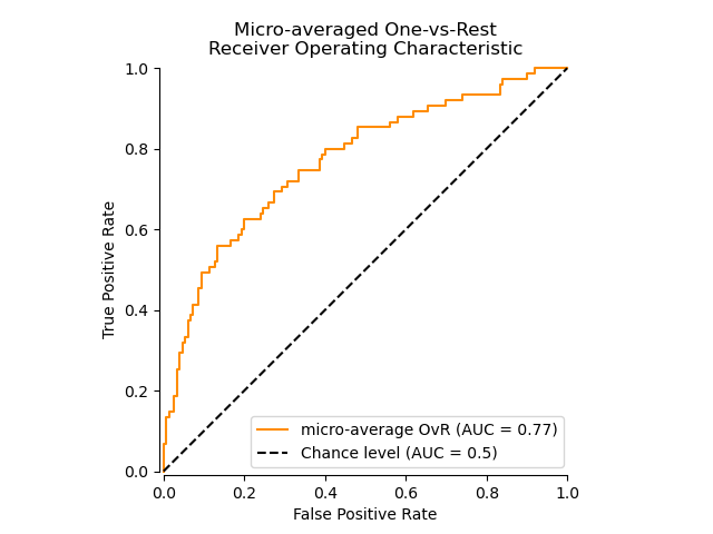

.

---

三、距离

.

1、海明距离

from sklearn.metrics import hamming_loss y_pred = [1, 2, 3, 4] y_true = [2, 2, 3, 4] hamming_loss(y_true, y_pred)0.25

.

2、Jaccard距离

 import numpy as np from sklearn.metrics import jaccard_similarity_score y_pred = [0, 2, 1, 3,4] y_true = [0, 1, 2, 3,4] jaccard_similarity_score(y_true, y_pred)0.5 jaccard_similarity_score(y_true, y_pred, normalize=False)2

.

---

四、回归

1、 可释方差值（Explained variance score）

 from sklearn.metrics import explained_variance_scorey_true = [3, -0.5, 2, 7] y_pred = [2.5, 0.0, 2, 8] explained_variance_score(y_true, y_pred)  

.

2、 平均绝对误差（Mean absolute error）

from sklearn.metrics import mean_absolute_error y_true = [3, -0.5, 2, 7] y_pred = [2.5, 0.0, 2, 8] mean_absolute_error(y_true, y_pred)

.

3、 均方误差（Mean squared error）

 from sklearn.metrics import mean_squared_error y_true = [3, -0.5, 2, 7] y_pred = [2.5, 0.0, 2, 8] mean_squared_error(y_true, y_pred)

.

4、中值绝对误差（Median absolute error）

 from sklearn.metrics import median_absolute_error y_true = [3, -0.5, 2, 7] y_pred = [2.5, 0.0, 2, 8] median_absolute_error(y_true, y_pred)

.

5、 R方值，确定系数

 from sklearn.metrics import r2_score y_true = [3, -0.5, 2, 7] y_pred = [2.5, 0.0, 2, 8] r2_score(y_true, y_pred)  

.

---

参考文献：

sklearn中的模型评估