10分钟Pandas教程

来源：互联网发布：java模拟发送get请求编辑：程序博客网时间：2024/05/22 04:57

10 Minutes to pandas

10分钟pandas教程

对于数据处理分析的新手，花十分钟熟悉pandas很有必要，一起开始吧~

第一步要会导入pandas和其好基友们：

In [1]: import pandas as pdIn [2]: import numpy as npIn [3]: import matplotlib.pyplot as plt

对象创建

本节可以具体参考Data Structure Intro section。

通过传入一个list的值来创建一个Series，并让pandas创建一个默认的序号索引：

In [4]: s = pd.Series([1,3,5,np.nan,6,8])In [5]: sOut[5]: 0    1.01    3.02    5.03    NaN4    6.05    8.0dtype: float64

通过传入一个numpy数组，创建一个DataFrame，并以时间为索引以列为标签：

In [6]: dates = pd.date_range('20130101', periods=6)In [7]: datesOut[7]: DatetimeIndex(['2013-01-01', '2013-01-02', '2013-01-03', '2013-01-04',               '2013-01-05', '2013-01-06'],              dtype='datetime64[ns]', freq='D')In [8]: df = pd.DataFrame(np.random.randn(6,4), index=dates, columns=list('ABCD'))In [9]: dfOut[9]:                    A         B         C         D2013-01-01  0.469112 -0.282863 -1.509059 -1.1356322013-01-02  1.212112 -0.173215  0.119209 -1.0442362013-01-03 -0.861849 -2.104569 -0.494929  1.0718042013-01-04  0.721555 -0.706771 -1.039575  0.2718602013-01-05 -0.424972  0.567020  0.276232 -1.0874012013-01-06 -0.673690  0.113648 -1.478427  0.524988

通过字典(dict)传入的对象而创建的DataFrame可以转为series样式：

In [10]: df2 = pd.DataFrame({ 'A' : 1.,   ....:                      'B' : pd.Timestamp('20130102'),   ....:                      'C' : pd.Series(1,index=list(range(4)),dtype='float32'),   ....:                      'D' : np.array([3] * 4,dtype='int32'),   ....:                      'E' : pd.Categorical(["test","train","test","train"]),   ....:                      'F' : 'foo' })   ....: In [11]: df2Out[11]:      A          B    C  D      E    F0  1.0 2013-01-02  1.0  3   test  foo1  1.0 2013-01-02  1.0  3  train  foo2  1.0 2013-01-02  1.0  3   test  foo3  1.0 2013-01-02  1.0  3  train  foo

其数据类型（dtypes）分别为：

In [12]: df2.dtypesOut[12]: A           float64B    datetime64[ns]C           float32D             int32E          categoryF            objectdtype: object

如果你在使用IPython，利用Tab键的自动补全会得到所有的列名称（除此外也有其他的公共属性）：

In [13]: df2.<TAB>df2.A                  df2.booldf2.abs                df2.boxplotdf2.add                df2.Cdf2.add_prefix         df2.clipdf2.add_suffix         df2.clip_lowerdf2.align              df2.clip_upperdf2.all                df2.columnsdf2.any                df2.combinedf2.append             df2.combine_firstdf2.apply              df2.compounddf2.applymap           df2.consolidatedf2.as_blocks          df2.convert_objectsdf2.asfreq             df2.copydf2.as_matrix          df2.corrdf2.astype             df2.corrwithdf2.at                 df2.countdf2.at_time            df2.covdf2.axes               df2.cummaxdf2.B                  df2.cummindf2.between_time       df2.cumproddf2.bfill              df2.cumsumdf2.blocks             df2.D

如你所见，A,B,C,D都被补全了，E也存在，但为了简洁被截断显示了。

浏览数据

详情参见Basics section。

查看frame中顶部和尾部行的数据：

In [14]: df.head()Out[14]:                    A         B         C         D2013-01-01  0.469112 -0.282863 -1.509059 -1.1356322013-01-02  1.212112 -0.173215  0.119209 -1.0442362013-01-03 -0.861849 -2.104569 -0.494929  1.0718042013-01-04  0.721555 -0.706771 -1.039575  0.2718602013-01-05 -0.424972  0.567020  0.276232 -1.087401In [15]: df.tail(3)Out[15]:                    A         B         C         D2013-01-04  0.721555 -0.706771 -1.039575  0.2718602013-01-05 -0.424972  0.567020  0.276232 -1.0874012013-01-06 -0.673690  0.113648 -1.478427  0.524988

显示索引，列标签，以及numpy格式的数据：

In [16]: df.indexOut[16]: DatetimeIndex(['2013-01-01', '2013-01-02', '2013-01-03', '2013-01-04',               '2013-01-05', '2013-01-06'],              dtype='datetime64[ns]', freq='D')In [17]: df.columnsOut[17]: Index(['A', 'B', 'C', 'D'], dtype='object')In [18]: df.valuesOut[18]: array([[ 0.4691, -0.2829, -1.5091, -1.1356],       [ 1.2121, -0.1732,  0.1192, -1.0442],       [-0.8618, -2.1046, -0.4949,  1.0718],       [ 0.7216, -0.7068, -1.0396,  0.2719],       [-0.425 ,  0.567 ,  0.2762, -1.0874],       [-0.6737,  0.1136, -1.4784,  0.525 ]])

对数据进行快速总结：

In [19]: df.describe()Out[19]:               A         B         C         Dcount  6.000000  6.000000  6.000000  6.000000mean   0.073711 -0.431125 -0.687758 -0.233103std    0.843157  0.922818  0.779887  0.973118min   -0.861849 -2.104569 -1.509059 -1.13563225%   -0.611510 -0.600794 -1.368714 -1.07661050%    0.022070 -0.228039 -0.767252 -0.38618875%    0.658444  0.041933 -0.034326  0.461706max    1.212112  0.567020  0.276232  1.071804

转置数据：

In [20]: df.TOut[20]:    2013-01-01  2013-01-02  2013-01-03  2013-01-04  2013-01-05  2013-01-06A    0.469112    1.212112   -0.861849    0.721555   -0.424972   -0.673690B   -0.282863   -0.173215   -2.104569   -0.706771    0.567020    0.113648C   -1.509059    0.119209   -0.494929   -1.039575    0.276232   -1.478427D   -1.135632   -1.044236    1.071804    0.271860   -1.087401    0.524988

按某一轴进行排序：

In [21]: df.sort_index(axis=1, ascending=False)Out[21]:                    D         C         B         A2013-01-01 -1.135632 -1.509059 -0.282863  0.4691122013-01-02 -1.044236  0.119209 -0.173215  1.2121122013-01-03  1.071804 -0.494929 -2.104569 -0.8618492013-01-04  0.271860 -1.039575 -0.706771  0.7215552013-01-05 -1.087401  0.276232  0.567020 -0.4249722013-01-06  0.524988 -1.478427  0.113648 -0.673690

按值排序：

In [22]: df.sort_values(by='B')Out[22]:                    A         B         C         D2013-01-03 -0.861849 -2.104569 -0.494929  1.0718042013-01-04  0.721555 -0.706771 -1.039575  0.2718602013-01-01  0.469112 -0.282863 -1.509059 -1.1356322013-01-02  1.212112 -0.173215  0.119209 -1.0442362013-01-06 -0.673690  0.113648 -1.478427  0.5249882013-01-05 -0.424972  0.567020  0.276232 -1.087401

选择

注意：虽然使用标准的Python/Numpy表达式进行选择和赋值是直观的，可以用于交互式工作，但对于生成代码，我们建议使用优化过的pandas数据访问方法：.at，.iat，.loc，.iloc和.ix。

获取

选择单独一列，返回一个Series，和df.A等同：

In [23]: df['A']Out[23]: 2013-01-01    0.4691122013-01-02    1.2121122013-01-03   -0.8618492013-01-04    0.7215552013-01-05   -0.4249722013-01-06   -0.673690Freq: D, Name: A, dtype: float64

使用[]选择，对行进行切片：

In [24]: df[0:3]Out[24]:                    A         B         C         D2013-01-01  0.469112 -0.282863 -1.509059 -1.1356322013-01-02  1.212112 -0.173215  0.119209 -1.0442362013-01-03 -0.861849 -2.104569 -0.494929  1.071804In [25]: df['20130102':'20130104']Out[25]:                    A         B         C         D2013-01-02  1.212112 -0.173215  0.119209 -1.0442362013-01-03 -0.861849 -2.104569 -0.494929  1.0718042013-01-04  0.721555 -0.706771 -1.039575  0.271860

用标签选择

参见Selection by Label。

使用标签选择得到一个交叉项：

In [26]: df.loc[dates[0]]Out[26]: A    0.469112B   -0.282863C   -1.509059D   -1.135632Name: 2013-01-01 00:00:00, dtype: float64

使用标签选择多个轴：

In [27]: df.loc[:,['A','B']]Out[27]:                    A         B2013-01-01  0.469112 -0.2828632013-01-02  1.212112 -0.1732152013-01-03 -0.861849 -2.1045692013-01-04  0.721555 -0.7067712013-01-05 -0.424972  0.5670202013-01-06 -0.673690  0.113648

显示标签切片，起止点都被包括在内：

In [28]: df.loc['20130102':'20130104',['A','B']]Out[28]:                    A         B2013-01-02  1.212112 -0.1732152013-01-03 -0.861849 -2.1045692013-01-04  0.721555 -0.706771

减少返回对象的维度：

In [29]: df.loc['20130102',['A','B']]Out[29]: A    1.212112B   -0.173215Name: 2013-01-02 00:00:00, dtype: float64

得到一个标量：

In [30]: df.loc[dates[0],'A']Out[30]: 0.46911229990718628

更快的速度！（和上面的方法一样）

In [31]: df.at[dates[0],'A']Out[31]: 0.46911229990718628

以位置选择

更多参见：Selection by Position

通过传入整数位置进行选择

In [32]: df.iloc[3]Out[32]: A    0.721555B   -0.706771C   -1.039575D    0.271860Name: 2013-01-04 00:00:00, dtype: float64

通过整数切片，和numpy、python的操作类似

In [33]: df.iloc[3:5,0:2]Out[33]:                    A         B2013-01-04  0.721555 -0.7067712013-01-05 -0.424972  0.567020

通过整数位置坐标，和numpy、python的风格类似：

In [34]: df.iloc[[1,2,4],[0,2]]Out[34]:                    A         C2013-01-02  1.212112  0.1192092013-01-03 -0.861849 -0.4949292013-01-05 -0.424972  0.276232

行切片：

In [35]: df.iloc[1:3,:]Out[35]:                    A         B         C         D2013-01-02  1.212112 -0.173215  0.119209 -1.0442362013-01-03 -0.861849 -2.104569 -0.494929  1.071804

列切片：

In [36]: df.iloc[:,1:3]Out[36]:                    B         C2013-01-01 -0.282863 -1.5090592013-01-02 -0.173215  0.1192092013-01-03 -2.104569 -0.4949292013-01-04 -0.706771 -1.0395752013-01-05  0.567020  0.2762322013-01-06  0.113648 -1.478427

获得某一点的值：

In [37]: df.iloc[1,1]Out[37]: -0.17321464905330858

更快的方法！

In [38]: df.iat[1,1]Out[38]: -0.17321464905330858

布尔值索引

使用单个列的（布尔）值进行选择：

In [39]: df[df.A > 0]Out[39]:                    A         B         C         D2013-01-01  0.469112 -0.282863 -1.509059 -1.1356322013-01-02  1.212112 -0.173215  0.119209 -1.0442362013-01-04  0.721555 -0.706771 -1.039575  0.271860

从一个DataFrame中，选择满足布尔条件的值：

In [40]: df[df > 0]Out[40]:                    A         B         C         D2013-01-01  0.469112       NaN       NaN       NaN2013-01-02  1.212112       NaN  0.119209       NaN2013-01-03       NaN       NaN       NaN  1.0718042013-01-04  0.721555       NaN       NaN  0.2718602013-01-05       NaN  0.567020  0.276232       NaN2013-01-06       NaN  0.113648       NaN  0.524988

使用isin()方法进行过滤：

In [41]: df2 = df.copy()In [42]: df2['E'] = ['one', 'one','two','three','four','three']In [43]: df2Out[43]:                    A         B         C         D      E2013-01-01  0.469112 -0.282863 -1.509059 -1.135632    one2013-01-02  1.212112 -0.173215  0.119209 -1.044236    one2013-01-03 -0.861849 -2.104569 -0.494929  1.071804    two2013-01-04  0.721555 -0.706771 -1.039575  0.271860  three2013-01-05 -0.424972  0.567020  0.276232 -1.087401   four2013-01-06 -0.673690  0.113648 -1.478427  0.524988  threeIn [44]: df2[df2['E'].isin(['two','four'])]Out[44]:                    A         B         C         D     E2013-01-03 -0.861849 -2.104569 -0.494929  1.071804   two2013-01-05 -0.424972  0.567020  0.276232 -1.087401  four

赋值

创建一个新的列，并自动使数据与索引对齐

In [45]: s1 = pd.Series([1,2,3,4,5,6], index=pd.date_range('20130102', periods=6))In [46]: s1Out[46]: 2013-01-02    12013-01-03    22013-01-04    32013-01-05    42013-01-06    52013-01-07    6Freq: D, dtype: int64In [47]: df['F'] = s1

通过标签赋值：

In [48]: df.at[dates[0],'A'] = 0

通过位置赋值：

In [49]: df.iat[0,1] = 0

通过指定的numpy数组赋值：

In [50]: df.loc[:,'D'] = np.array([5] * len(df))In [51]: dfOut[51]:                    A         B         C  D    F2013-01-01  0.000000  0.000000 -1.509059  5  NaN2013-01-02  1.212112 -0.173215  0.119209  5  1.02013-01-03 -0.861849 -2.104569 -0.494929  5  2.02013-01-04  0.721555 -0.706771 -1.039575  5  3.02013-01-05 -0.424972  0.567020  0.276232  5  4.02013-01-06 -0.673690  0.113648 -1.478427  5  5.0

使用where操作赋值：

In [52]: df2 = df.copy()In [53]: df2[df2 > 0] = -df2In [54]: df2Out[54]:                    A         B         C  D    F2013-01-01  0.000000  0.000000 -1.509059 -5  NaN2013-01-02 -1.212112 -0.173215 -0.119209 -5 -1.02013-01-03 -0.861849 -2.104569 -0.494929 -5 -2.02013-01-04 -0.721555 -0.706771 -1.039575 -5 -3.02013-01-05 -0.424972 -0.567020 -0.276232 -5 -4.02013-01-06 -0.673690 -0.113648 -1.478427 -5 -5.0

缺失数据

pandas主要使用np.nan来表示缺失的数据。它默认不被计算所包括。详见：Missing Data section。

重新索引允许更改/添加/删除指定轴上的索引。这将返回该数据的副本。

In [55]: df1 = df.reindex(index=dates[0:4], columns=list(df.columns) + ['E'])In [56]: df1.loc[dates[0]:dates[1],'E'] = 1In [57]: df1Out[57]:                    A         B         C  D    F    E2013-01-01  0.000000  0.000000 -1.509059  5  NaN  1.02013-01-02  1.212112 -0.173215  0.119209  5  1.0  1.02013-01-03 -0.861849 -2.104569 -0.494929  5  2.0  NaN2013-01-04  0.721555 -0.706771 -1.039575  5  3.0  NaN

丢弃任意拥有缺失数据的列：

In [58]: df1.dropna(how='any')Out[58]:                    A         B         C  D    F    E2013-01-02  1.212112 -0.173215  0.119209  5  1.0  1.0

填充缺失数据：

In [59]: df1.fillna(value=5)Out[59]:                    A         B         C  D    F    E2013-01-01  0.000000  0.000000 -1.509059  5  5.0  1.02013-01-02  1.212112 -0.173215  0.119209  5  1.0  1.02013-01-03 -0.861849 -2.104569 -0.494929  5  2.0  5.02013-01-04  0.721555 -0.706771 -1.039575  5  3.0  5.0

获得布尔值掩模当数据为nan时：

In [60]: pd.isnull(df1)Out[60]:                 A      B      C      D      F      E2013-01-01  False  False  False  False   True  False2013-01-02  False  False  False  False  False  False2013-01-03  False  False  False  False  False   True2013-01-04  False  False  False  False  False   True

操作：

详见Basic section on Binary Ops

统计值

通常情况下不包括缺失数据。

描述性统计：

In [61]: df.mean()Out[61]: A   -0.004474B   -0.383981C   -0.687758D    5.000000F    3.000000dtype: float64

对某一轴进行同样的操作：

In [62]: df.mean(1)Out[62]: 2013-01-01    0.8727352013-01-02    1.4316212013-01-03    0.7077312013-01-04    1.3950422013-01-05    1.8836562013-01-06    1.592306Freq: D, dtype: float64

对于拥有不同维度的对象，操作需要进行对齐。pandas会自动沿着选定的维度进行broadcasts。

In [63]: s = pd.Series([1,3,5,np.nan,6,8], index=dates).shift(2)In [64]: sOut[64]: 2013-01-01    NaN2013-01-02    NaN2013-01-03    1.02013-01-04    3.02013-01-05    5.02013-01-06    NaNFreq: D, dtype: float64In [65]: df.sub(s, axis='index')Out[65]:                    A         B         C    D    F2013-01-01       NaN       NaN       NaN  NaN  NaN2013-01-02       NaN       NaN       NaN  NaN  NaN2013-01-03 -1.861849 -3.104569 -1.494929  4.0  1.02013-01-04 -2.278445 -3.706771 -4.039575  2.0  0.02013-01-05 -5.424972 -4.432980 -4.723768  0.0 -1.02013-01-06       NaN       NaN       NaN  NaN  NaN

应用

对数据应用函数：

In [66]: df.apply(np.cumsum)Out[66]:                    A         B         C   D     F2013-01-01  0.000000  0.000000 -1.509059   5   NaN2013-01-02  1.212112 -0.173215 -1.389850  10   1.02013-01-03  0.350263 -2.277784 -1.884779  15   3.02013-01-04  1.071818 -2.984555 -2.924354  20   6.02013-01-05  0.646846 -2.417535 -2.648122  25  10.02013-01-06 -0.026844 -2.303886 -4.126549  30  15.0In [67]: df.apply(lambda x: x.max() - x.min())Out[67]: A    2.073961B    2.671590C    1.785291D    0.000000F    4.000000dtype: float64

直方图

详见直方图Histogramming and Discretization。

In [68]: s = pd.Series(np.random.randint(0, 7, size=10))In [69]: sOut[69]: 0    41    22    13    24    65    46    47    68    49    4dtype: int64In [70]: s.value_counts()Out[70]: 4    56    22    21    1dtype: int64

字符串方法

series 在 str属性中具有许多操作，模式匹配通常使用正则表达式。更多参见 Vectorized String Methods。

In [71]: s = pd.Series(['A', 'B', 'C', 'Aaba', 'Baca', np.nan, 'CABA', 'dog', 'cat'])In [72]: s.str.lower()Out[72]: 0       a1       b2       c3    aaba4    baca5     NaN6    caba7     dog8     catdtype: object

合并

连接

pandas提供了多种利用逻辑关系合并 Series, DataFrame, 和 Panel 对象的简易方法。详见Merging section。

连接pandas对象使用concat()。

In [73]: df = pd.DataFrame(np.random.randn(10, 4))In [74]: dfOut[74]:           0         1         2         30 -0.548702  1.467327 -1.015962 -0.4830751  1.637550 -1.217659 -0.291519 -1.7455052 -0.263952  0.991460 -0.919069  0.2660463 -0.709661  1.669052  1.037882 -1.7057754 -0.919854 -0.042379  1.247642 -0.0099205  0.290213  0.495767  0.362949  1.5481066 -1.131345 -0.089329  0.337863 -0.9458677 -0.932132  1.956030  0.017587 -0.0166928 -0.575247  0.254161 -1.143704  0.2158979  1.193555 -0.077118 -0.408530 -0.862495# break it into piecesIn [75]: pieces = [df[:3], df[3:7], df[7:]]In [76]: pd.concat(pieces)Out[76]:           0         1         2         30 -0.548702  1.467327 -1.015962 -0.4830751  1.637550 -1.217659 -0.291519 -1.7455052 -0.263952  0.991460 -0.919069  0.2660463 -0.709661  1.669052  1.037882 -1.7057754 -0.919854 -0.042379  1.247642 -0.0099205  0.290213  0.495767  0.362949  1.5481066 -1.131345 -0.089329  0.337863 -0.9458677 -0.932132  1.956030  0.017587 -0.0166928 -0.575247  0.254161 -1.143704  0.2158979  1.193555 -0.077118 -0.408530 -0.862495

加入

SQL式的合并。参见Database style joining

In [77]: left = pd.DataFrame({'key': ['foo', 'foo'], 'lval': [1, 2]})In [78]: right = pd.DataFrame({'key': ['foo', 'foo'], 'rval': [4, 5]})In [79]: leftOut[79]:    key  lval0  foo     11  foo     2In [80]: rightOut[80]:    key  rval0  foo     41  foo     5In [81]: pd.merge(left, right, on='key')Out[81]:    key  lval  rval0  foo     1     41  foo     1     52  foo     2     43  foo     2     5

添加

在Dataframe上添加一行。详见 Appending。

In [87]: df = pd.DataFrame(np.random.randn(8, 4), columns=['A','B','C','D'])In [88]: dfOut[88]:           A         B         C         D0  1.346061  1.511763  1.627081 -0.9905821 -0.441652  1.211526  0.268520  0.0245802 -1.577585  0.396823 -0.105381 -0.5325323  1.453749  1.208843 -0.080952 -0.2646104 -0.727965 -0.589346  0.339969 -0.6932055 -0.339355  0.593616  0.884345  1.5914316  0.141809  0.220390  0.435589  0.1924517 -0.096701  0.803351  1.715071 -0.708758In [89]: s = df.iloc[3]In [90]: df.append(s, ignore_index=True)Out[90]:           A         B         C         D0  1.346061  1.511763  1.627081 -0.9905821 -0.441652  1.211526  0.268520  0.0245802 -1.577585  0.396823 -0.105381 -0.5325323  1.453749  1.208843 -0.080952 -0.2646104 -0.727965 -0.589346  0.339969 -0.6932055 -0.339355  0.593616  0.884345  1.5914316  0.141809  0.220390  0.435589  0.1924517 -0.096701  0.803351  1.715071 -0.7087588  1.453749  1.208843 -0.080952 -0.264610

分组

分组指的是以下一或多个步骤：

分割按不同的规则分割数据
应用对每组应用不同的函数
结合将结果结合到一个数据类型

详见Grouping section

In [91]: df = pd.DataFrame({'A' : ['foo', 'bar', 'foo', 'bar',   ....:                           'foo', 'bar', 'foo', 'foo'],   ....:                    'B' : ['one', 'one', 'two', 'three',   ....:                           'two', 'two', 'one', 'three'],   ....:                    'C' : np.random.randn(8),   ....:                    'D' : np.random.randn(8)})   ....: In [92]: dfOut[92]:      A      B         C         D0  foo    one -1.202872 -0.0552241  bar    one -1.814470  2.3959852  foo    two  1.018601  1.5528253  bar  three -0.595447  0.1665994  foo    two  1.395433  0.0476095  bar    two -0.392670 -0.1364736  foo    one  0.007207 -0.5617577  foo  three  1.928123 -1.623033

使用sum函数对分组对象进行求和。

In [93]: df.groupby('A').sum()Out[93]:             C        DA                     bar -2.802588  2.42611foo  3.146492 -0.63958

使用多个列标签进行分组：

In [94]: df.groupby(['A','B']).sum()Out[94]:                   C         DA   B                        bar one   -1.814470  2.395985    three -0.595447  0.166599    two   -0.392670 -0.136473foo one   -1.195665 -0.616981    three  1.928123 -1.623033    two    2.414034  1.600434

变形

详见Hierarchical Indexing 和 Reshaping。

Stack

In [95]: tuples = list(zip(*[['bar', 'bar', 'baz', 'baz',   ....:                      'foo', 'foo', 'qux', 'qux'],   ....:                     ['one', 'two', 'one', 'two',   ....:                      'one', 'two', 'one', 'two']]))   ....: In [96]: index = pd.MultiIndex.from_tuples(tuples, names=['first', 'second'])In [97]: df = pd.DataFrame(np.random.randn(8, 2), index=index, columns=['A', 'B'])In [98]: df2 = df[:4]In [99]: df2Out[99]:                      A         Bfirst second                    bar   one     0.029399 -0.542108      two     0.282696 -0.087302baz   one    -1.575170  1.771208      two     0.816482  1.100230

stack()方法将DataFrame压缩为一列。

In [100]: stacked = df2.stack()In [101]: stackedOut[101]: first  second   bar    one     A    0.029399               B   -0.542108       two     A    0.282696               B   -0.087302baz    one     A   -1.575170               B    1.771208       two     A    0.816482               B    1.100230dtype: float64

逆操作为 unstack()。

In [102]: stacked.unstack()Out[102]:                      A         Bfirst second                    bar   one     0.029399 -0.542108      two     0.282696 -0.087302baz   one    -1.575170  1.771208      two     0.816482  1.100230In [103]: stacked.unstack(1)Out[103]: second        one       twofirst                      bar   A  0.029399  0.282696      B -0.542108 -0.087302baz   A -1.575170  0.816482      B  1.771208  1.100230In [104]: stacked.unstack(0)Out[104]: first          bar       bazsecond                      one    A  0.029399 -1.575170       B -0.542108  1.771208two    A  0.282696  0.816482       B -0.087302  1.100230

数据透视表

详见 Pivot Tables。

In [105]: df = pd.DataFrame({'A' : ['one', 'one', 'two', 'three'] * 3,   .....:                    'B' : ['A', 'B', 'C'] * 4,   .....:                    'C' : ['foo', 'foo', 'foo', 'bar', 'bar', 'bar'] * 2,   .....:                    'D' : np.random.randn(12),   .....:                    'E' : np.random.randn(12)})   .....: In [106]: dfOut[106]:         A  B    C         D         E0     one  A  foo  1.418757 -0.1796661     one  B  foo -1.879024  1.2918362     two  C  foo  0.536826 -0.0096143   three  A  bar  1.006160  0.3921494     one  B  bar -0.029716  0.2645995     one  C  bar -1.146178 -0.0574096     two  A  foo  0.100900 -1.4256387   three  B  foo -1.035018  1.0240988     one  C  foo  0.314665 -0.1060629     one  A  bar -0.773723  1.82437510    two  B  bar -1.170653  0.59597411  three  C  bar  0.648740  1.167115

可以很简单地产生透视表：

In [107]: pd.pivot_table(df, values='D', index=['A', 'B'], columns=['C'])Out[107]: C             bar       fooA     B                    one   A -0.773723  1.418757      B -0.029716 -1.879024      C -1.146178  0.314665three A  1.006160       NaN      B       NaN -1.035018      C  0.648740       NaNtwo   A       NaN  0.100900      B -1.170653       NaN      C       NaN  0.536826

时间序列

pandas具有简单、强大以及有效的时间序列函数，详见Time Series section。

In [108]: rng = pd.date_range('1/1/2012', periods=100, freq='S')In [109]: ts = pd.Series(np.random.randint(0, 500, len(rng)), index=rng)In [110]: ts.resample('5Min').sum()Out[110]: 2012-01-01    25083Freq: 5T, dtype: int64

时区转换：

In [111]: rng = pd.date_range('3/6/2012 00:00', periods=5, freq='D')In [112]: ts = pd.Series(np.random.randn(len(rng)), rng)In [113]: tsOut[113]: 2012-03-06    0.4640002012-03-07    0.2273712012-03-08   -0.4969222012-03-09    0.3063892012-03-10   -2.290613Freq: D, dtype: float64In [114]: ts_utc = ts.tz_localize('UTC')In [115]: ts_utcOut[115]: 2012-03-06 00:00:00+00:00    0.4640002012-03-07 00:00:00+00:00    0.2273712012-03-08 00:00:00+00:00   -0.4969222012-03-09 00:00:00+00:00    0.3063892012-03-10 00:00:00+00:00   -2.290613Freq: D, dtype: float64

转为另一个时区

In [116]: ts_utc.tz_convert('US/Eastern')Out[116]: 2012-03-05 19:00:00-05:00    0.4640002012-03-06 19:00:00-05:00    0.2273712012-03-07 19:00:00-05:00   -0.4969222012-03-08 19:00:00-05:00    0.3063892012-03-09 19:00:00-05:00   -2.290613Freq: D, dtype: float64

时区跨度表示：

In [117]: rng = pd.date_range('1/1/2012', periods=5, freq='M')In [118]: ts = pd.Series(np.random.randn(len(rng)), index=rng)In [119]: tsOut[119]: 2012-01-31   -1.1346232012-02-29   -1.5618192012-03-31   -0.2608382012-04-30    0.2819572012-05-31    1.523962Freq: M, dtype: float64In [120]: ps = ts.to_period()In [121]: psOut[121]: 2012-01   -1.1346232012-02   -1.5618192012-03   -0.2608382012-04    0.2819572012-05    1.523962Freq: M, dtype: float64In [122]: ps.to_timestamp()Out[122]: 2012-01-01   -1.1346232012-02-01   -1.5618192012-03-01   -0.2608382012-04-01    0.2819572012-05-01    1.523962Freq: MS, dtype: float64

周期和时间戳的转换让算数函数变得方便。

In [123]: prng = pd.period_range('1990Q1', '2000Q4', freq='Q-NOV')In [124]: ts = pd.Series(np.random.randn(len(prng)), prng)In [125]: ts.index = (prng.asfreq('M', 'e') + 1).asfreq('H', 's') + 9In [126]: ts.head()Out[126]: 1990-03-01 09:00   -0.9029371990-06-01 09:00    0.0681591990-09-01 09:00   -0.0578731990-12-01 09:00   -0.3682041991-03-01 09:00   -1.144073Freq: H, dtype: float64

分类

从0.15版本开始，pandas可以在DataFrame中支持Categorical类型的数据，详细介绍参看：categorical introduction和API documentation。

In [127]: df = pd.DataFrame({"id":[1,2,3,4,5,6], "raw_grade":['a', 'b', 'b', 'a', 'a', 'e']})

把原始等级转为分类类型。

In [128]: df["grade"] = df["raw_grade"].astype("category")In [129]: df["grade"]Out[129]: 0    a1    b2    b3    a4    a5    eName: grade, dtype: categoryCategories (3, object): [a, b, e]

重命名类名：

In [130]: df["grade"].cat.categories = ["very good", "good", "very bad"]

分类重新排序：

In [131]: df["grade"] = df["grade"].cat.set_categories(["very bad", "bad", "medium", "good", "very good"])In [132]: df["grade"]Out[132]: 0    very good1         good2         good3    very good4    very good5     very badName: grade, dtype: categoryCategories (5, object): [very bad, bad, medium, good, very good]

数据以类别排序：

In [133]: df.sort_values(by="grade")Out[133]:    id raw_grade      grade5   6         e   very bad1   2         b       good2   3         b       good0   1         a  very good3   4         a  very good4   5         a  very good

使用分组并包括空目录分类：

In [134]: df.groupby("grade").size()Out[134]: gradevery bad     1bad          0medium       0good         2very good    3dtype: int64

绘图

绘图文档参见Plotting

In [135]: ts = pd.Series(np.random.randn(1000), index=pd.date_range('1/1/2000', periods=1000))In [136]: ts = ts.cumsum()In [137]: ts.plot()Out[137]: <matplotlib.axes._subplots.AxesSubplot at 0x1187d7278>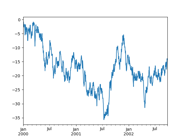

plot

在DataFrame中，plot()是一种以列为标签绘图的简单方法。

In [138]: df = pd.DataFrame(np.random.randn(1000, 4), index=ts.index,   .....:                   columns=['A', 'B', 'C', 'D'])   .....: In [139]: df = df.cumsum()In [140]: plt.figure(); df.plot(); plt.legend(loc='best')Out[140]: <matplotlib.legend.Legend at 0x11b5dea20>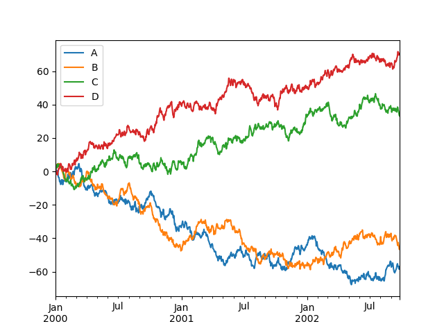

plot1

Getting Data In/Out

CSV

写一个csv文件。

In [141]: df.to_csv('foo.csv')

读一个csv文件。

In [142]: pd.read_csv('foo.csv')Out[142]:      Unnamed: 0          A          B         C          D0    2000-01-01   0.266457  -0.399641 -0.219582   1.1868601    2000-01-02  -1.170732  -0.345873  1.653061  -0.2829532    2000-01-03  -1.734933   0.530468  2.060811  -0.5155363    2000-01-04  -1.555121   1.452620  0.239859  -1.1568964    2000-01-05   0.578117   0.511371  0.103552  -2.4282025    2000-01-06   0.478344   0.449933 -0.741620  -1.9624096    2000-01-07   1.235339  -0.091757 -1.543861  -1.084753..          ...        ...        ...       ...        ...993  2002-09-20 -10.628548  -9.153563 -7.883146  28.313940994  2002-09-21 -10.390377  -8.727491 -6.399645  30.914107995  2002-09-22  -8.985362  -8.485624 -4.669462  31.367740996  2002-09-23  -9.558560  -8.781216 -4.499815  30.518439997  2002-09-24  -9.902058  -9.340490 -4.386639  30.105593998  2002-09-25 -10.216020  -9.480682 -3.933802  29.758560999  2002-09-26 -11.856774 -10.671012 -3.216025  29.369368[1000 rows x 5 columns]

HDF5

读写HDFStores。

写：

In [143]: df.to_hdf('foo.h5','df')

读：

In [144]: pd.read_hdf('foo.h5','df')Out[144]:                     A          B         C          D2000-01-01   0.266457  -0.399641 -0.219582   1.1868602000-01-02  -1.170732  -0.345873  1.653061  -0.2829532000-01-03  -1.734933   0.530468  2.060811  -0.5155362000-01-04  -1.555121   1.452620  0.239859  -1.1568962000-01-05   0.578117   0.511371  0.103552  -2.4282022000-01-06   0.478344   0.449933 -0.741620  -1.9624092000-01-07   1.235339  -0.091757 -1.543861  -1.084753...               ...        ...       ...        ...2002-09-20 -10.628548  -9.153563 -7.883146  28.3139402002-09-21 -10.390377  -8.727491 -6.399645  30.9141072002-09-22  -8.985362  -8.485624 -4.669462  31.3677402002-09-23  -9.558560  -8.781216 -4.499815  30.5184392002-09-24  -9.902058  -9.340490 -4.386639  30.1055932002-09-25 -10.216020  -9.480682 -3.933802  29.7585602002-09-26 -11.856774 -10.671012 -3.216025  29.369368[1000 rows x 4 columns]

Excel

读写MS Excel。

写：

In [145]: df.to_excel('foo.xlsx', sheet_name='Sheet1')

读：

In [146]: pd.read_excel('foo.xlsx', 'Sheet1', index_col=None, na_values=['NA'])Out[146]:                     A          B         C          D2000-01-01   0.266457  -0.399641 -0.219582   1.1868602000-01-02  -1.170732  -0.345873  1.653061  -0.2829532000-01-03  -1.734933   0.530468  2.060811  -0.5155362000-01-04  -1.555121   1.452620  0.239859  -1.1568962000-01-05   0.578117   0.511371  0.103552  -2.4282022000-01-06   0.478344   0.449933 -0.741620  -1.9624092000-01-07   1.235339  -0.091757 -1.543861  -1.084753...               ...        ...       ...        ...2002-09-20 -10.628548  -9.153563 -7.883146  28.3139402002-09-21 -10.390377  -8.727491 -6.399645  30.9141072002-09-22  -8.985362  -8.485624 -4.669462  31.3677402002-09-23  -9.558560  -8.781216 -4.499815  30.5184392002-09-24  -9.902058  -9.340490 -4.386639  30.1055932002-09-25 -10.216020  -9.480682 -3.933802  29.7585602002-09-26 -11.856774 -10.671012 -3.216025  29.369368[1000 rows x 4 columns]

　陷阱

>>> if pd.Series([False, True, False]):    print("I was true")Traceback    ...ValueError: The truth value of an array is ambiguous. Use a.empty, a.any() or a.all().

阅读全文

1 0