This is a short introduction to pandas, geared mainly for new users. You can see more complex recipes in theCookbook
Object Creation
See the Data Structure Intro section
Creating a Series by passing a list of values, letting pandas create a default integer index:
In [4]: s = pd.Series([1,3,5,np.nan,6,8])In [5]: sOut[5]: 0 1.01 3.02 5.03 NaN4 6.05 8.0dtype: float64
Creating a DataFrame by passing a numpy array, with a datetime index and labeled columns:
In [6]: dates = pd.date_range('20130101', periods=6)In [7]: datesOut[7]: DatetimeIndex(['2013-01-01', '2013-01-02', '2013-01-03', '2013-01-04', '2013-01-05', '2013-01-06'], dtype='datetime64[ns]', freq='D')In [8]: df = pd.DataFrame(np.random.randn(6,4), index=dates, columns=list('ABCD'))In [9]: dfOut[9]: A B C D2013-01-01 0.469112 -0.282863 -1.509059 -1.1356322013-01-02 1.212112 -0.173215 0.119209 -1.0442362013-01-03 -0.861849 -2.104569 -0.494929 1.0718042013-01-04 0.721555 -0.706771 -1.039575 0.2718602013-01-05 -0.424972 0.567020 0.276232 -1.0874012013-01-06 -0.673690 0.113648 -1.478427 0.524988Creating a DataFrame by passing a dict of objects that can be converted to series-like.
In [10]: df2 = pd.DataFrame({ 'A' : 1., ....: 'B' : pd.Timestamp('20130102'), ....: 'C' : pd.Series(1,index=list(range(4)),dtype='float32'), ....: 'D' : np.array([3] * 4,dtype='int32'), ....: 'E' : pd.Categorical(["test","train","test","train"]), ....: 'F' : 'foo' }) ....: In [11]: df2Out[11]: A B C D E F0 1.0 2013-01-02 1.0 3 test foo1 1.0 2013-01-02 1.0 3 train foo2 1.0 2013-01-02 1.0 3 test foo3 1.0 2013-01-02 1.0 3 train fooHaving specific dtypes
In [12]: df2.dtypesOut[12]: A float64B datetime64[ns]C float32D int32E categoryF objectdtype: object
If you’re using IPython, tab completion for column names (as well as public attributes) is automatically enabled. Here’s a subset of the attributes that will be completed:
In [13]: df2.<TAB>df2.A df2.boxplotdf2.abs df2.Cdf2.add df2.clipdf2.add_prefix df2.clip_lowerdf2.add_suffix df2.clip_upperdf2.align df2.columnsdf2.all df2.combinedf2.any df2.combineAdddf2.append df2.combine_firstdf2.apply df2.combineMultdf2.applymap df2.compounddf2.as_blocks df2.consolidatedf2.asfreq df2.convert_objectsdf2.as_matrix df2.copydf2.astype df2.corrdf2.at df2.corrwithdf2.at_time df2.countdf2.axes df2.covdf2.B df2.cummaxdf2.between_time df2.cummindf2.bfill df2.cumproddf2.blocks df2.cumsumdf2.bool df2.D
As you can see, the columns A, B, C, and D are automatically tab completed. E is there as well; the rest of the attributes have been truncated for brevity.
Viewing Data
See the Basics section
See the top & bottom rows of the frame
In [14]: df.head()Out[14]: A B C D2013-01-01 0.469112 -0.282863 -1.509059 -1.1356322013-01-02 1.212112 -0.173215 0.119209 -1.0442362013-01-03 -0.861849 -2.104569 -0.494929 1.0718042013-01-04 0.721555 -0.706771 -1.039575 0.2718602013-01-05 -0.424972 0.567020 0.276232 -1.087401In [15]: df.tail(3)Out[15]: A B C D2013-01-04 0.721555 -0.706771 -1.039575 0.2718602013-01-05 -0.424972 0.567020 0.276232 -1.0874012013-01-06 -0.673690 0.113648 -1.478427 0.524988
Display the index, columns, and the underlying numpy data
In [16]: df.indexOut[16]: DatetimeIndex(['2013-01-01', '2013-01-02', '2013-01-03', '2013-01-04', '2013-01-05', '2013-01-06'], dtype='datetime64[ns]', freq='D')In [17]: df.columnsOut[17]: Index([u'A', u'B', u'C', u'D'], dtype='object')In [18]: df.valuesOut[18]: array([[ 0.4691, -0.2829, -1.5091, -1.1356], [ 1.2121, -0.1732, 0.1192, -1.0442], [-0.8618, -2.1046, -0.4949, 1.0718], [ 0.7216, -0.7068, -1.0396, 0.2719], [-0.425 , 0.567 , 0.2762, -1.0874], [-0.6737, 0.1136, -1.4784, 0.525 ]])
Describe shows a quick statistic summary of your data
In [19]: df.describe()Out[19]: A B C Dcount 6.000000 6.000000 6.000000 6.000000mean 0.073711 -0.431125 -0.687758 -0.233103std 0.843157 0.922818 0.779887 0.973118min -0.861849 -2.104569 -1.509059 -1.13563225% -0.611510 -0.600794 -1.368714 -1.07661050% 0.022070 -0.228039 -0.767252 -0.38618875% 0.658444 0.041933 -0.034326 0.461706max 1.212112 0.567020 0.276232 1.071804
Transposing your data
In [20]: df.TOut[20]: 2013-01-01 2013-01-02 2013-01-03 2013-01-04 2013-01-05 2013-01-06A 0.469112 1.212112 -0.861849 0.721555 -0.424972 -0.673690B -0.282863 -0.173215 -2.104569 -0.706771 0.567020 0.113648C -1.509059 0.119209 -0.494929 -1.039575 0.276232 -1.478427D -1.135632 -1.044236 1.071804 0.271860 -1.087401 0.524988
Sorting by an axis
In [21]: df.sort_index(axis=1, ascending=False)Out[21]: D C B A2013-01-01 -1.135632 -1.509059 -0.282863 0.4691122013-01-02 -1.044236 0.119209 -0.173215 1.2121122013-01-03 1.071804 -0.494929 -2.104569 -0.8618492013-01-04 0.271860 -1.039575 -0.706771 0.7215552013-01-05 -1.087401 0.276232 0.567020 -0.4249722013-01-06 0.524988 -1.478427 0.113648 -0.673690
Sorting by values
In [22]: df.sort_values(by='B')Out[22]: A B C D2013-01-03 -0.861849 -2.104569 -0.494929 1.0718042013-01-04 0.721555 -0.706771 -1.039575 0.2718602013-01-01 0.469112 -0.282863 -1.509059 -1.1356322013-01-02 1.212112 -0.173215 0.119209 -1.0442362013-01-06 -0.673690 0.113648 -1.478427 0.5249882013-01-05 -0.424972 0.567020 0.276232 -1.087401
Selection
Note
While standard Python / Numpy expressions for selecting and setting are intuitive and come in handy for interactive work, for production code, we recommend the optimized pandas data access methods, .at, .iat, .loc,.iloc and .ix.
See the indexing documentation Indexing and Selecting Data and MultiIndex / Advanced Indexing
Getting
Selecting a single column, which yields a Series, equivalent to df.A
In [23]: df['A']Out[23]: 2013-01-01 0.4691122013-01-02 1.2121122013-01-03 -0.8618492013-01-04 0.7215552013-01-05 -0.4249722013-01-06 -0.673690Freq: D, Name: A, dtype: float64
Selecting via [], which slices the rows.
In [24]: df[0:3]Out[24]: A B C D2013-01-01 0.469112 -0.282863 -1.509059 -1.1356322013-01-02 1.212112 -0.173215 0.119209 -1.0442362013-01-03 -0.861849 -2.104569 -0.494929 1.071804In [25]: df['20130102':'20130104']Out[25]: A B C D2013-01-02 1.212112 -0.173215 0.119209 -1.0442362013-01-03 -0.861849 -2.104569 -0.494929 1.0718042013-01-04 0.721555 -0.706771 -1.039575 0.271860
Selection by Label
See more in Selection by Label
For getting a cross section using a label
In [26]: df.loc[dates[0]]Out[26]: A 0.469112B -0.282863C -1.509059D -1.135632Name: 2013-01-01 00:00:00, dtype: float64
Selecting on a multi-axis by label
In [27]: df.loc[:,['A','B']]Out[27]: A B2013-01-01 0.469112 -0.2828632013-01-02 1.212112 -0.1732152013-01-03 -0.861849 -2.1045692013-01-04 0.721555 -0.7067712013-01-05 -0.424972 0.5670202013-01-06 -0.673690 0.113648
Showing label slicing, both endpoints are included
In [28]: df.loc['20130102':'20130104',['A','B']]Out[28]: A B2013-01-02 1.212112 -0.1732152013-01-03 -0.861849 -2.1045692013-01-04 0.721555 -0.706771
Reduction in the dimensions of the returned object
In [29]: df.loc['20130102',['A','B']]Out[29]: A 1.212112B -0.173215Name: 2013-01-02 00:00:00, dtype: float64
For getting a scalar value
In [30]: df.loc[dates[0],'A']Out[30]: 0.46911229990718628
For getting fast access to a scalar (equiv to the prior method)
In [31]: df.at[dates[0],'A']Out[31]: 0.46911229990718628
Selection by Position
See more in Selection by Position
Select via the position of the passed integers
In [32]: df.iloc[3]Out[32]: A 0.721555B -0.706771C -1.039575D 0.271860Name: 2013-01-04 00:00:00, dtype: float64
By integer slices, acting similar to numpy/python
In [33]: df.iloc[3:5,0:2]Out[33]: A B2013-01-04 0.721555 -0.7067712013-01-05 -0.424972 0.567020
By lists of integer position locations, similar to the numpy/python style
In [34]: df.iloc[[1,2,4],[0,2]]Out[34]: A C2013-01-02 1.212112 0.1192092013-01-03 -0.861849 -0.4949292013-01-05 -0.424972 0.276232
For slicing rows explicitly
In [35]: df.iloc[1:3,:]Out[35]: A B C D2013-01-02 1.212112 -0.173215 0.119209 -1.0442362013-01-03 -0.861849 -2.104569 -0.494929 1.071804
For slicing columns explicitly
In [36]: df.iloc[:,1:3]Out[36]: B C2013-01-01 -0.282863 -1.5090592013-01-02 -0.173215 0.1192092013-01-03 -2.104569 -0.4949292013-01-04 -0.706771 -1.0395752013-01-05 0.567020 0.2762322013-01-06 0.113648 -1.478427
For getting a value explicitly
In [37]: df.iloc[1,1]Out[37]: -0.17321464905330858
For getting fast access to a scalar (equiv to the prior method)
In [38]: df.iat[1,1]Out[38]: -0.17321464905330858
Boolean Indexing
Using a single column’s values to select data.
In [39]: df[df.A > 0]Out[39]: A B C D2013-01-01 0.469112 -0.282863 -1.509059 -1.1356322013-01-02 1.212112 -0.173215 0.119209 -1.0442362013-01-04 0.721555 -0.706771 -1.039575 0.271860
A where operation for getting.
In [40]: df[df > 0]Out[40]: A B C D2013-01-01 0.469112 NaN NaN NaN2013-01-02 1.212112 NaN 0.119209 NaN2013-01-03 NaN NaN NaN 1.0718042013-01-04 0.721555 NaN NaN 0.2718602013-01-05 NaN 0.567020 0.276232 NaN2013-01-06 NaN 0.113648 NaN 0.524988
Using the isin() method for filtering:
In [41]: df2 = df.copy()In [42]: df2['E'] = ['one', 'one','two','three','four','three']In [43]: df2Out[43]: A B C D E2013-01-01 0.469112 -0.282863 -1.509059 -1.135632 one2013-01-02 1.212112 -0.173215 0.119209 -1.044236 one2013-01-03 -0.861849 -2.104569 -0.494929 1.071804 two2013-01-04 0.721555 -0.706771 -1.039575 0.271860 three2013-01-05 -0.424972 0.567020 0.276232 -1.087401 four2013-01-06 -0.673690 0.113648 -1.478427 0.524988 threeIn [44]: df2[df2['E'].isin(['two','four'])]Out[44]: A B C D E2013-01-03 -0.861849 -2.104569 -0.494929 1.071804 two2013-01-05 -0.424972 0.567020 0.276232 -1.087401 four
Setting
Setting a new column automatically aligns the data by the indexes
In [45]: s1 = pd.Series([1,2,3,4,5,6], index=pd.date_range('20130102', periods=6))In [46]: s1Out[46]: 2013-01-02 12013-01-03 22013-01-04 32013-01-05 42013-01-06 52013-01-07 6Freq: D, dtype: int64In [47]: df['F'] = s1Setting values by label
In [48]: df.at[dates[0],'A'] = 0
Setting values by position
Setting by assigning with a numpy array
In [50]: df.loc[:,'D'] = np.array([5] * len(df))
The result of the prior setting operations
In [51]: dfOut[51]: A B C D F2013-01-01 0.000000 0.000000 -1.509059 5 NaN2013-01-02 1.212112 -0.173215 0.119209 5 1.02013-01-03 -0.861849 -2.104569 -0.494929 5 2.02013-01-04 0.721555 -0.706771 -1.039575 5 3.02013-01-05 -0.424972 0.567020 0.276232 5 4.02013-01-06 -0.673690 0.113648 -1.478427 5 5.0
A where operation with setting.
In [52]: df2 = df.copy()In [53]: df2[df2 > 0] = -df2In [54]: df2Out[54]: A B C D F2013-01-01 0.000000 0.000000 -1.509059 -5 NaN2013-01-02 -1.212112 -0.173215 -0.119209 -5 -1.02013-01-03 -0.861849 -2.104569 -0.494929 -5 -2.02013-01-04 -0.721555 -0.706771 -1.039575 -5 -3.02013-01-05 -0.424972 -0.567020 -0.276232 -5 -4.02013-01-06 -0.673690 -0.113648 -1.478427 -5 -5.0
Missing Data
pandas primarily uses the value np.nan to represent missing data. It is by default not included in computations. See the Missing Data section
Reindexing allows you to change/add/delete the index on a specified axis. This returns a copy of the data.
In [55]: df1 = df.reindex(index=dates[0:4], columns=list(df.columns) + ['E'])In [56]: df1.loc[dates[0]:dates[1],'E'] = 1In [57]: df1Out[57]: A B C D F E2013-01-01 0.000000 0.000000 -1.509059 5 NaN 1.02013-01-02 1.212112 -0.173215 0.119209 5 1.0 1.02013-01-03 -0.861849 -2.104569 -0.494929 5 2.0 NaN2013-01-04 0.721555 -0.706771 -1.039575 5 3.0 NaN
To drop any rows that have missing data.
In [58]: df1.dropna(how='any')Out[58]: A B C D F E2013-01-02 1.212112 -0.173215 0.119209 5 1.0 1.0
Filling missing data
In [59]: df1.fillna(value=5)Out[59]: A B C D F E2013-01-01 0.000000 0.000000 -1.509059 5 5.0 1.02013-01-02 1.212112 -0.173215 0.119209 5 1.0 1.02013-01-03 -0.861849 -2.104569 -0.494929 5 2.0 5.02013-01-04 0.721555 -0.706771 -1.039575 5 3.0 5.0
To get the boolean mask where values are nan
In [60]: pd.isnull(df1)Out[60]: A B C D F E2013-01-01 False False False False True False2013-01-02 False False False False False False2013-01-03 False False False False False True2013-01-04 False False False False False True
Operations
See the Basic section on Binary Ops
Stats
Operations in general exclude missing data.
Performing a descriptive statistic
In [61]: df.mean()Out[61]: A -0.004474B -0.383981C -0.687758D 5.000000F 3.000000dtype: float64
Same operation on the other axis
In [62]: df.mean(1)Out[62]: 2013-01-01 0.8727352013-01-02 1.4316212013-01-03 0.7077312013-01-04 1.3950422013-01-05 1.8836562013-01-06 1.592306Freq: D, dtype: float64
Operating with objects that have different dimensionality and need alignment. In addition, pandas automatically broadcasts along the specified dimension.
In [63]: s = pd.Series([1,3,5,np.nan,6,8], index=dates).shift(2)In [64]: sOut[64]: 2013-01-01 NaN2013-01-02 NaN2013-01-03 1.02013-01-04 3.02013-01-05 5.02013-01-06 NaNFreq: D, dtype: float64In [65]: df.sub(s, axis='index')Out[65]: A B C D F2013-01-01 NaN NaN NaN NaN NaN2013-01-02 NaN NaN NaN NaN NaN2013-01-03 -1.861849 -3.104569 -1.494929 4.0 1.02013-01-04 -2.278445 -3.706771 -4.039575 2.0 0.02013-01-05 -5.424972 -4.432980 -4.723768 0.0 -1.02013-01-06 NaN NaN NaN NaN NaN
Apply
Applying functions to the data
In [66]: df.apply(np.cumsum)Out[66]: A B C D F2013-01-01 0.000000 0.000000 -1.509059 5 NaN2013-01-02 1.212112 -0.173215 -1.389850 10 1.02013-01-03 0.350263 -2.277784 -1.884779 15 3.02013-01-04 1.071818 -2.984555 -2.924354 20 6.02013-01-05 0.646846 -2.417535 -2.648122 25 10.02013-01-06 -0.026844 -2.303886 -4.126549 30 15.0In [67]: df.apply(lambda x: x.max() - x.min())Out[67]: A 2.073961B 2.671590C 1.785291D 0.000000F 4.000000dtype: float64
Histogramming
See more at Histogramming and Discretization
In [68]: s = pd.Series(np.random.randint(0, 7, size=10))In [69]: sOut[69]: 0 41 22 13 24 65 46 47 68 49 4dtype: int64In [70]: s.value_counts()Out[70]: 4 56 22 21 1dtype: int64
String Methods
Series is equipped with a set of string processing methods in the str attribute that make it easy to operate on each element of the array, as in the code snippet below. Note that pattern-matching in str generally uses regular expressions by default (and in some cases always uses them). See more at Vectorized String Methods.
In [71]: s = pd.Series(['A', 'B', 'C', 'Aaba', 'Baca', np.nan, 'CABA', 'dog', 'cat'])In [72]: s.str.lower()Out[72]: 0 a1 b2 c3 aaba4 baca5 NaN6 caba7 dog8 catdtype: object
Merge
Concat
pandas provides various facilities for easily combining together Series, DataFrame, and Panel objects with various kinds of set logic for the indexes and relational algebra functionality in the case of join / merge-type operations.
See the Merging section
Concatenating pandas objects together with concat():
In [73]: df = pd.DataFrame(np.random.randn(10, 4))In [74]: dfOut[74]: 0 1 2 30 -0.548702 1.467327 -1.015962 -0.4830751 1.637550 -1.217659 -0.291519 -1.7455052 -0.263952 0.991460 -0.919069 0.2660463 -0.709661 1.669052 1.037882 -1.7057754 -0.919854 -0.042379 1.247642 -0.0099205 0.290213 0.495767 0.362949 1.5481066 -1.131345 -0.089329 0.337863 -0.9458677 -0.932132 1.956030 0.017587 -0.0166928 -0.575247 0.254161 -1.143704 0.2158979 1.193555 -0.077118 -0.408530 -0.862495# break it into piecesIn [75]: pieces = [df[:3], df[3:7], df[7:]]In [76]: pd.concat(pieces)Out[76]: 0 1 2 30 -0.548702 1.467327 -1.015962 -0.4830751 1.637550 -1.217659 -0.291519 -1.7455052 -0.263952 0.991460 -0.919069 0.2660463 -0.709661 1.669052 1.037882 -1.7057754 -0.919854 -0.042379 1.247642 -0.0099205 0.290213 0.495767 0.362949 1.5481066 -1.131345 -0.089329 0.337863 -0.9458677 -0.932132 1.956030 0.017587 -0.0166928 -0.575247 0.254161 -1.143704 0.2158979 1.193555 -0.077118 -0.408530 -0.862495
Join
SQL style merges. See the Database style joining
In [77]: left = pd.DataFrame({'key': ['foo', 'foo'], 'lval': [1, 2]})In [78]: right = pd.DataFrame({'key': ['foo', 'foo'], 'rval': [4, 5]})In [79]: leftOut[79]: key lval0 foo 11 foo 2In [80]: rightOut[80]: key rval0 foo 41 foo 5In [81]: pd.merge(left, right, on='key')Out[81]: key lval rval0 foo 1 41 foo 1 52 foo 2 43 foo 2 5Another example that can be given is:
In [82]: left = pd.DataFrame({'key': ['foo', 'bar'], 'lval': [1, 2]})In [83]: right = pd.DataFrame({'key': ['foo', 'bar'], 'rval': [4, 5]})In [84]: leftOut[84]: key lval0 foo 11 bar 2In [85]: rightOut[85]: key rval0 foo 41 bar 5In [86]: pd.merge(left, right, on='key')Out[86]: key lval rval0 foo 1 41 bar 2 5Append
Append rows to a dataframe. See the Appending
In [87]: df = pd.DataFrame(np.random.randn(8, 4), columns=['A','B','C','D'])In [88]: dfOut[88]: A B C D0 1.346061 1.511763 1.627081 -0.9905821 -0.441652 1.211526 0.268520 0.0245802 -1.577585 0.396823 -0.105381 -0.5325323 1.453749 1.208843 -0.080952 -0.2646104 -0.727965 -0.589346 0.339969 -0.6932055 -0.339355 0.593616 0.884345 1.5914316 0.141809 0.220390 0.435589 0.1924517 -0.096701 0.803351 1.715071 -0.708758In [89]: s = df.iloc[3]In [90]: df.append(s, ignore_index=True)Out[90]: A B C D0 1.346061 1.511763 1.627081 -0.9905821 -0.441652 1.211526 0.268520 0.0245802 -1.577585 0.396823 -0.105381 -0.5325323 1.453749 1.208843 -0.080952 -0.2646104 -0.727965 -0.589346 0.339969 -0.6932055 -0.339355 0.593616 0.884345 1.5914316 0.141809 0.220390 0.435589 0.1924517 -0.096701 0.803351 1.715071 -0.7087588 1.453749 1.208843 -0.080952 -0.264610
Grouping
By “group by” we are referring to a process involving one or more of the following steps
- Splitting the data into groups based on some criteria
- Applying a function to each group independently
- Combining the results into a data structure
See the Grouping section
In [91]: df = pd.DataFrame({'A' : ['foo', 'bar', 'foo', 'bar', ....: 'foo', 'bar', 'foo', 'foo'], ....: 'B' : ['one', 'one', 'two', 'three', ....: 'two', 'two', 'one', 'three'], ....: 'C' : np.random.randn(8), ....: 'D' : np.random.randn(8)}) ....: In [92]: dfOut[92]: A B C D0 foo one -1.202872 -0.0552241 bar one -1.814470 2.3959852 foo two 1.018601 1.5528253 bar three -0.595447 0.1665994 foo two 1.395433 0.0476095 bar two -0.392670 -0.1364736 foo one 0.007207 -0.5617577 foo three 1.928123 -1.623033Grouping and then applying a function sum to the resulting groups.
In [93]: df.groupby('A').sum()Out[93]: C DA bar -2.802588 2.42611foo 3.146492 -0.63958Grouping by multiple columns forms a hierarchical index, which we then apply the function.
In [94]: df.groupby(['A','B']).sum()Out[94]: C DA B bar one -1.814470 2.395985 three -0.595447 0.166599 two -0.392670 -0.136473foo one -1.195665 -0.616981 three 1.928123 -1.623033 two 2.414034 1.600434
Reshaping
See the sections on Hierarchical Indexing and Reshaping.
Stack
In [95]: tuples = list(zip(*[['bar', 'bar', 'baz', 'baz', ....: 'foo', 'foo', 'qux', 'qux'], ....: ['one', 'two', 'one', 'two', ....: 'one', 'two', 'one', 'two']])) ....: In [96]: index = pd.MultiIndex.from_tuples(tuples, names=['first', 'second'])In [97]: df = pd.DataFrame(np.random.randn(8, 2), index=index, columns=['A', 'B'])In [98]: df2 = df[:4]In [99]: df2Out[99]: A Bfirst second bar one 0.029399 -0.542108 two 0.282696 -0.087302baz one -1.575170 1.771208 two 0.816482 1.100230
The stack() method “compresses” a level in the DataFrame’s columns.
In [100]: stacked = df2.stack()In [101]: stackedOut[101]: first second bar one A 0.029399 B -0.542108 two A 0.282696 B -0.087302baz one A -1.575170 B 1.771208 two A 0.816482 B 1.100230dtype: float64
With a “stacked” DataFrame or Series (having a MultiIndex as the index), the inverse operation of stack() is unstack(), which by default unstacks the last level:
In [102]: stacked.unstack()Out[102]: A Bfirst second bar one 0.029399 -0.542108 two 0.282696 -0.087302baz one -1.575170 1.771208 two 0.816482 1.100230In [103]: stacked.unstack(1)Out[103]: second one twofirst bar A 0.029399 0.282696 B -0.542108 -0.087302baz A -1.575170 0.816482 B 1.771208 1.100230In [104]: stacked.unstack(0)Out[104]: first bar bazsecond one A 0.029399 -1.575170 B -0.542108 1.771208two A 0.282696 0.816482 B -0.087302 1.100230
Pivot Tables
See the section on Pivot Tables.
In [105]: df = pd.DataFrame({'A' : ['one', 'one', 'two', 'three'] * 3, .....: 'B' : ['A', 'B', 'C'] * 4, .....: 'C' : ['foo', 'foo', 'foo', 'bar', 'bar', 'bar'] * 2, .....: 'D' : np.random.randn(12), .....: 'E' : np.random.randn(12)}) .....: In [106]: dfOut[106]: A B C D E0 one A foo 1.418757 -0.1796661 one B foo -1.879024 1.2918362 two C foo 0.536826 -0.0096143 three A bar 1.006160 0.3921494 one B bar -0.029716 0.2645995 one C bar -1.146178 -0.0574096 two A foo 0.100900 -1.4256387 three B foo -1.035018 1.0240988 one C foo 0.314665 -0.1060629 one A bar -0.773723 1.82437510 two B bar -1.170653 0.59597411 three C bar 0.648740 1.167115We can produce pivot tables from this data very easily:
In [107]: pd.pivot_table(df, values='D', index=['A', 'B'], columns=['C'])Out[107]: C bar fooA B one A -0.773723 1.418757 B -0.029716 -1.879024 C -1.146178 0.314665three A 1.006160 NaN B NaN -1.035018 C 0.648740 NaNtwo A NaN 0.100900 B -1.170653 NaN C NaN 0.536826
Time Series
pandas has simple, powerful, and efficient functionality for performing resampling operations during frequency conversion (e.g., converting secondly data into 5-minutely data). This is extremely common in, but not limited to, financial applications. See the Time Series section
In [108]: rng = pd.date_range('1/1/2012', periods=100, freq='S')In [109]: ts = pd.Series(np.random.randint(0, 500, len(rng)), index=rng)In [110]: ts.resample('5Min').sum()Out[110]: 2012-01-01 25083Freq: 5T, dtype: int64Time zone representation
In [111]: rng = pd.date_range('3/6/2012 00:00', periods=5, freq='D')In [112]: ts = pd.Series(np.random.randn(len(rng)), rng)In [113]: tsOut[113]: 2012-03-06 0.4640002012-03-07 0.2273712012-03-08 -0.4969222012-03-09 0.3063892012-03-10 -2.290613Freq: D, dtype: float64In [114]: ts_utc = ts.tz_localize('UTC')In [115]: ts_utcOut[115]: 2012-03-06 00:00:00+00:00 0.4640002012-03-07 00:00:00+00:00 0.2273712012-03-08 00:00:00+00:00 -0.4969222012-03-09 00:00:00+00:00 0.3063892012-03-10 00:00:00+00:00 -2.290613Freq: D, dtype: float64Convert to another time zone
In [116]: ts_utc.tz_convert('US/Eastern')Out[116]: 2012-03-05 19:00:00-05:00 0.4640002012-03-06 19:00:00-05:00 0.2273712012-03-07 19:00:00-05:00 -0.4969222012-03-08 19:00:00-05:00 0.3063892012-03-09 19:00:00-05:00 -2.290613Freq: D, dtype: float64Converting between time span representations
In [117]: rng = pd.date_range('1/1/2012', periods=5, freq='M')In [118]: ts = pd.Series(np.random.randn(len(rng)), index=rng)In [119]: tsOut[119]: 2012-01-31 -1.1346232012-02-29 -1.5618192012-03-31 -0.2608382012-04-30 0.2819572012-05-31 1.523962Freq: M, dtype: float64In [120]: ps = ts.to_period()In [121]: psOut[121]: 2012-01 -1.1346232012-02 -1.5618192012-03 -0.2608382012-04 0.2819572012-05 1.523962Freq: M, dtype: float64In [122]: ps.to_timestamp()Out[122]: 2012-01-01 -1.1346232012-02-01 -1.5618192012-03-01 -0.2608382012-04-01 0.2819572012-05-01 1.523962Freq: MS, dtype: float64Converting between period and timestamp enables some convenient arithmetic functions to be used. In the following example, we convert a quarterly frequency with year ending in November to 9am of the end of the month following the quarter end:
In [123]: prng = pd.period_range('1990Q1', '2000Q4', freq='Q-NOV')In [124]: ts = pd.Series(np.random.randn(len(prng)), prng)In [125]: ts.index = (prng.asfreq('M', 'e') + 1).asfreq('H', 's') + 9In [126]: ts.head()Out[126]: 1990-03-01 09:00 -0.9029371990-06-01 09:00 0.0681591990-09-01 09:00 -0.0578731990-12-01 09:00 -0.3682041991-03-01 09:00 -1.144073Freq: H, dtype: float64Categoricals
Since version 0.15, pandas can include categorical data in a DataFrame. For full docs, see the categorical introductionand the API documentation.
In [127]: df = pd.DataFrame({"id":[1,2,3,4,5,6], "raw_grade":['a', 'b', 'b', 'a', 'a', 'e']})Convert the raw grades to a categorical data type.
In [128]: df["grade"] = df["raw_grade"].astype("category")In [129]: df["grade"]Out[129]: 0 a1 b2 b3 a4 a5 eName: grade, dtype: categoryCategories (3, object): [a, b, e]Rename the categories to more meaningful names (assigning to Series.cat.categories is inplace!)
In [130]: df["grade"].cat.categories = ["very good", "good", "very bad"]
Reorder the categories and simultaneously add the missing categories (methods under Series .cat return a newSeries per default).
In [131]: df["grade"] = df["grade"].cat.set_categories(["very bad", "bad", "medium", "good", "very good"])In [132]: df["grade"]Out[132]: 0 very good1 good2 good3 very good4 very good5 very badName: grade, dtype: categoryCategories (5, object): [very bad, bad, medium, good, very good]
Sorting is per order in the categories, not lexical order.
In [133]: df.sort_values(by="grade")Out[133]: id raw_grade grade5 6 e very bad1 2 b good2 3 b good0 1 a very good3 4 a very good4 5 a very good
Grouping by a categorical column shows also empty categories.
In [134]: df.groupby("grade").size()Out[134]: gradevery bad 1bad 0medium 0good 2very good 3dtype: int64Plotting
Plotting docs.
In [135]: ts = pd.Series(np.random.randn(1000), index=pd.date_range('1/1/2000', periods=1000))In [136]: ts = ts.cumsum()In [137]: ts.plot()Out[137]: <matplotlib.axes._subplots.AxesSubplot at 0x7f3df3e049d0>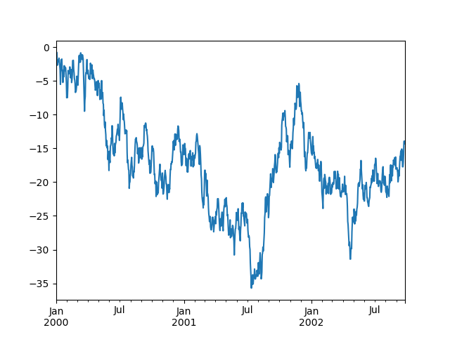
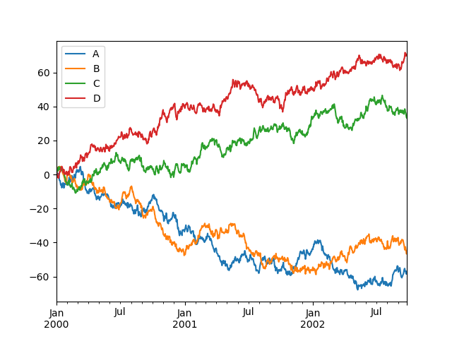
On DataFrame, plot() is a convenience to plot all of the columns with labels:
In [138]: df = pd.DataFrame(np.random.randn(1000, 4), index=ts.index, .....: columns=['A', 'B', 'C', 'D']) .....: In [139]: df = df.cumsum()In [140]: plt.figure(); df.plot(); plt.legend(loc='best')Out[140]: <matplotlib.legend.Legend at 0x7f3de816b7d0>
Getting Data In/Out
CSV
Writing to a csv file
In [141]: df.to_csv('foo.csv')Reading from a csv file
In [142]: pd.read_csv('foo.csv')Out[142]: Unnamed: 0 A B C D0 2000-01-01 0.266457 -0.399641 -0.219582 1.1868601 2000-01-02 -1.170732 -0.345873 1.653061 -0.2829532 2000-01-03 -1.734933 0.530468 2.060811 -0.5155363 2000-01-04 -1.555121 1.452620 0.239859 -1.1568964 2000-01-05 0.578117 0.511371 0.103552 -2.4282025 2000-01-06 0.478344 0.449933 -0.741620 -1.9624096 2000-01-07 1.235339 -0.091757 -1.543861 -1.084753.. ... ... ... ... ...993 2002-09-20 -10.628548 -9.153563 -7.883146 28.313940994 2002-09-21 -10.390377 -8.727491 -6.399645 30.914107995 2002-09-22 -8.985362 -8.485624 -4.669462 31.367740996 2002-09-23 -9.558560 -8.781216 -4.499815 30.518439997 2002-09-24 -9.902058 -9.340490 -4.386639 30.105593998 2002-09-25 -10.216020 -9.480682 -3.933802 29.758560999 2002-09-26 -11.856774 -10.671012 -3.216025 29.369368[1000 rows x 5 columns]HDF5
Reading and writing to HDFStores
Writing to a HDF5 Store
In [143]: df.to_hdf('foo.h5','df')Reading from a HDF5 Store
In [144]: pd.read_hdf('foo.h5','df')Out[144]: A B C D2000-01-01 0.266457 -0.399641 -0.219582 1.1868602000-01-02 -1.170732 -0.345873 1.653061 -0.2829532000-01-03 -1.734933 0.530468 2.060811 -0.5155362000-01-04 -1.555121 1.452620 0.239859 -1.1568962000-01-05 0.578117 0.511371 0.103552 -2.4282022000-01-06 0.478344 0.449933 -0.741620 -1.9624092000-01-07 1.235339 -0.091757 -1.543861 -1.084753... ... ... ... ...2002-09-20 -10.628548 -9.153563 -7.883146 28.3139402002-09-21 -10.390377 -8.727491 -6.399645 30.9141072002-09-22 -8.985362 -8.485624 -4.669462 31.3677402002-09-23 -9.558560 -8.781216 -4.499815 30.5184392002-09-24 -9.902058 -9.340490 -4.386639 30.1055932002-09-25 -10.216020 -9.480682 -3.933802 29.7585602002-09-26 -11.856774 -10.671012 -3.216025 29.369368[1000 rows x 4 columns]Excel
Reading and writing to MS Excel
Writing to an excel file
In [145]: df.to_excel('foo.xlsx', sheet_name='Sheet1')Reading from an excel file
In [146]: pd.read_excel('foo.xlsx', 'Sheet1', index_col=None, na_values=['NA'])Out[146]: A B C D2000-01-01 0.266457 -0.399641 -0.219582 1.1868602000-01-02 -1.170732 -0.345873 1.653061 -0.2829532000-01-03 -1.734933 0.530468 2.060811 -0.5155362000-01-04 -1.555121 1.452620 0.239859 -1.1568962000-01-05 0.578117 0.511371 0.103552 -2.4282022000-01-06 0.478344 0.449933 -0.741620 -1.9624092000-01-07 1.235339 -0.091757 -1.543861 -1.084753... ... ... ... ...2002-09-20 -10.628548 -9.153563 -7.883146 28.3139402002-09-21 -10.390377 -8.727491 -6.399645 30.9141072002-09-22 -8.985362 -8.485624 -4.669462 31.3677402002-09-23 -9.558560 -8.781216 -4.499815 30.5184392002-09-24 -9.902058 -9.340490 -4.386639 30.1055932002-09-25 -10.216020 -9.480682 -3.933802 29.7585602002-09-26 -11.856774 -10.671012 -3.216025 29.369368[1000 rows x 4 columns]Gotchas
If you are trying an operation and you see an exception like:
>>> if pd.Series([False, True, False]): print("I was true")Traceback ...ValueError: The truth value of an array is ambiguous. Use a.empty, a.any() or a.all().See Comparisons for an explanation and what to do.
See Gotchas as well.