A Guide For Time Series Prediction Using Recurrent Neural Networks (LSTMs)

Forecasting future currency exchange rates with long short-term memory (LSTMs)

The Statsbot team has already published the article about using time series analysis for anomaly detection. Today, we’d like to discuss time series prediction with a long short-term memory model (LSTMs). We asked a data scientist, Neelabh Pant, to tell you about his experience of forecasting exchange rates using recurrent neural networks.As an Indian guy living in the US, I have a constant flow of money from home to me and vice versa. If the USD is stronger in the market, then the Indian rupee (INR) goes down, hence, a person from India buys a dollar for more rupees. If the dollar is weaker, you spend less rupees to buy the same dollar.

If one can predict how much a dollar will cost tomorrow, then this can guide one’s decision making and can be very important in minimizing risks and maximizing returns. Looking at the strengths of a neural network, especially a recurrent neural network, I came up with the idea of predicting the exchange rate between the USD and the INR.

There are a lot of methods of forecasting exchange rates such as:

• Purchasing Power Parity (PPP), which takes the inflation into account and calculates inflation differential.
• Relative Economic Strength Approach, which considers the economic growth of countries to predict the direction of exchange rates.
• Econometric model is another common technique used to forecast the exchange rates which is customizable according to the factors or attributes the forecaster thinks are important. There could be features like interest rate differential between two different countries, GDP growth rates, income growth rates, etc.
• Time series model is purely dependent on the idea that past behavior and price patterns can be used to predict future price behavior.

In this article, we’ll tell you how to predict the future exchange rate behavior using time series analysis and by making use of machine learning with time series.

Sequence problems

Let us begin by talking about sequence problems. The simplest machine learning problem involving a sequence is a one to one problem.

One to One

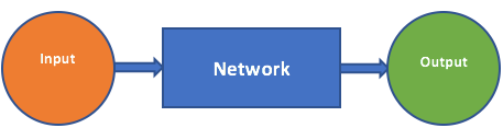
In this case, we have one data input or tensor to the model and the model generates a prediction with the given input. Linear regression, classification, and even image classification with convolutional network fall into this category. We can extend this formulation to allow for the model to make use of the pass values of the input and the output.

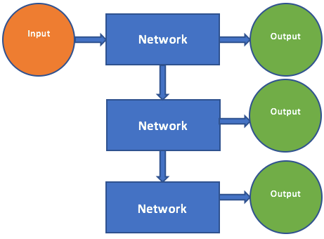
It is known as the one to many problem. The one to many problem starts like the one to one problem where we have an input to the model and the model generates one output. However, the output of the model is now fed back to the model as a new input. The model now can generate a new output and we can continue like this indefinitely. You can now see why these are known as recurrent neural networks.

One to Many

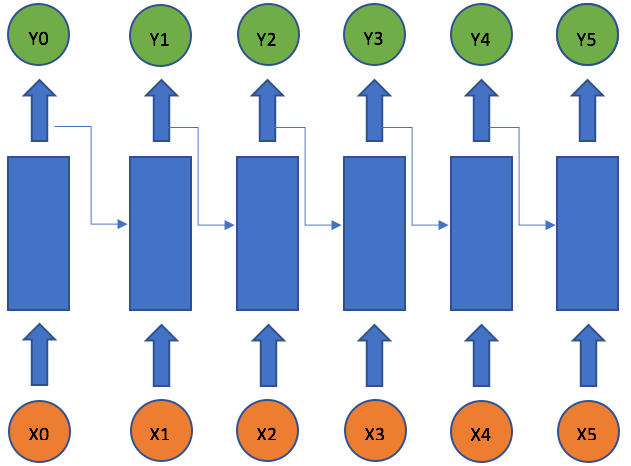
A recurrent neural network deals with sequence problems because their connections form a directed cycle. In other words, they can retain state from one iteration to the next by using their own output as input for the next step. In programming terms this is like running a fixed program with certain inputs and some internal variables. The simplest recurrent neural network can be viewed as a fully connected neural network if we unroll the time axes.

RNN Unrolled Time

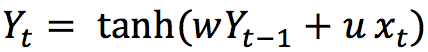
In this univariate case only two weights are involved. The weight multiplying the current input xt, which is u, and the weight multiplying the previous output yt-1, which is w. This formula is like the exponential weighted moving average (EWMA) by making its pass values of the output with the current values of the input.

One can build a deep recurrent neural network by simply stacking units to one another. A simple recurrent neural network works well only for a short-term memory. We will see that it suffers from a fundamental problem if we have a longer time dependency.

Long Short-Term Neural Network

As we have talked about, a simple recurrent network suffers from a fundamental problem of not being able to capture long-term dependencies in a sequence. This is a problem because we want our RNNs to analyze text and answer questions, which involves keeping track of long sequences of words.

In late ’90s, LSTM was proposed by Sepp Hochreiter and Jurgen Schmidhuber, which is relatively insensitive to gap length over alternatives RNNs, hidden markov models, and other sequence learning methods in numerous applications.

LSTM Architecture

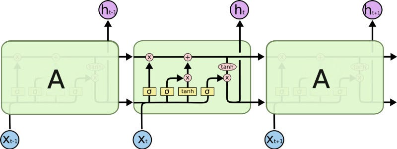
This model is organized in cells which include several operations. LSTM has an internal state variable, which is passed from one cell to another and modified by Operation Gates.

1. Forget Gate

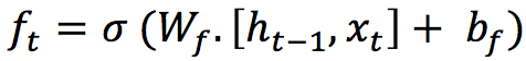
It is a sigmoid layer that takes the output at t-1 and the current input at time t and concatenates them into a single tensor and applies a linear transformation followed by a sigmoid. Because of the sigmoid, the output of this gate is between 0 and 1. This number is multiplied with the internal state and that is why the gate is called a forget gate. If ft=0 then the previous internal state is completely forgotten, while if ft=1 it will be passed through unaltered.

2. Input Gate

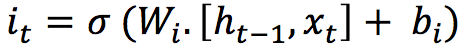
The input gate takes the previous output and the new input and passes them through another sigmoid layer. This gate returns a value between 0 and 1. The value of the input gate is multiplied with the output of the candidate layer.

This layer applies a hyperbolic tangent to the mix of input and previous output, returning a candidate vector to be added to the internal state.

The internal state is updated with this rule:

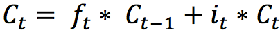
.The previous state is multiplied by the forget gate and then added to the fraction of the new candidate allowed by the output gate.

3. Output Gate

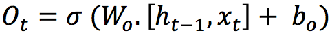
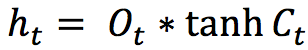
This gate controls how much of the internal state is passed to the output and it works in a similar way to the other gates.

These three gates described above have independent weights and biases, hence the network will learn how much of the past output to keep, how much of the current input to keep, and how much of the internal state to send out to the output.

In a recurrent neural network, you not only give the network the data, but also the state of the network one moment before. For example, if I say “Hey! Something crazy happened to me when I was driving” there is a part of your brain that is flipping a switch that’s saying “Oh, this is a story Neelabh is telling me. It is a story where the main character is Neelabh and something happened on the road.” Now, you carry a little part of that one sentence I just told you. As you listen to all my other sentences you have to keep a bit of information from all past sentences around in order to understand the entire story.

Another example is video processing, where you would again need a recurrent neural network. What happens in the current frame is heavily dependent upon what was in the last frame of the movie most of the time. Over a period of time, a recurrent neural network tries to learn what to keep and how much to keep from the past, and how much information to keep from the present state, which makes it so powerful as compared to a simple feed forward neural network.

Time Series Prediction

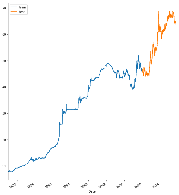
I was impressed with the strengths of a recurrent neural network and decided to use them to predict the exchange rate between the USD and the INR. The dataset used in this project is the exchange rate data between January 2, 1980 and August 10, 2017. Later, I’ll give you a link to download this dataset and experiment with it.

Table 1. Dataset Example

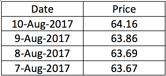
The dataset displays the value of $1 in rupees. We have a total of 13,730 records starting from January 2, 1980 to August 10, 2017.

USD vs INR

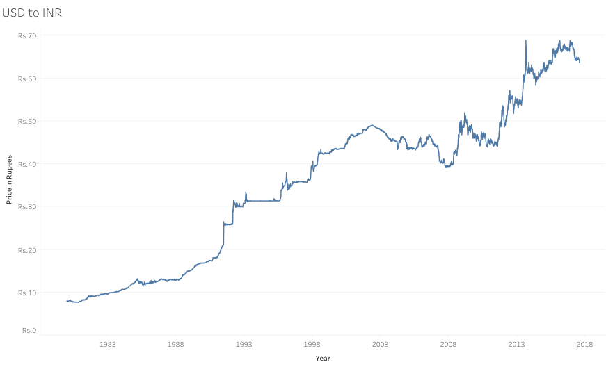
Over the period, the price to buy $1 in rupees has been rising. One can see that there was a huge dip in the American economy during 2007–2008, which was hugely caused by the great recession during that period. It was a period of general economic decline observed in world markets during the late 2000s and early 2010s.

This period was not very good for the world’s developed economies, particularly in North America and Europe (including Russia), which fell into a definitive recession. Many of the newer developed economies suffered far less impact, particularly China and India, whose economies grew substantially during this period.

Test-Train Split

Now, to train the machine we need to divide the dataset into test and training sets. It is very important when you do time series to split train and test with respect to a certain date. So, you don’t want your test data to come before your training data.

In our experiment, we will define a date, say January 1, 2010, as our split date. The training data is the data between January 2, 1980 and December 31, 2009, which are about 11,000 training data points.

The test dataset is between January 1, 2010 and August 10, 2017, which are about 2,700 points.

Train-Test Split

The next thing to do is normalize the dataset. You only need to fit and transform your training data and just transform your test data. The reason you do that is you don’t want to assume that you know the scale of your test data.

Normalizing or transforming the data means that the new scale variables will be between zero and one.

Neural Network Models

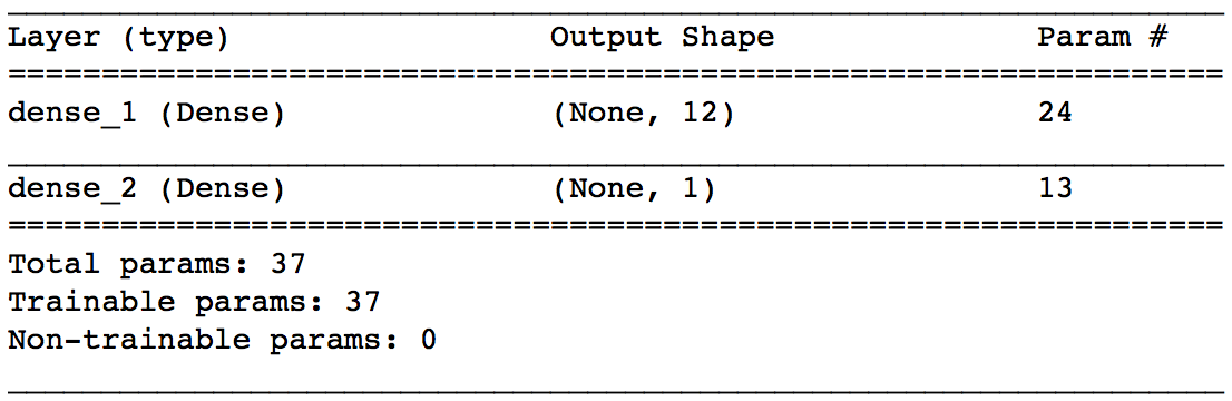
A fully Connected Model is a simple neural network model which is built as a simple regression model that will take one input and will spit out one output. This basically takes the price from the previous day and forecasts the price of the next day.

As a loss function, we use mean squared error and stochastic gradient descent as an optimizer, which after enough numbers of epochs will try to look for a good local optimum. Below is the summary of the fully connected layer.

Summary of a Fully Connected Layer

After training this model for 200 epochs or early_callbacks (whichever came first), the model tries to learn the pattern and the behavior of the data. Since we split the data into training and testing sets we can now predict the value of testing data and compare them with the ground truth.

Ground Truth(blue) vs Prediction(orange)

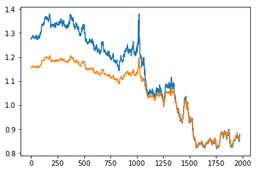
As you can see, the model is not good. It essentially is repeating the previous values and there is a slight shift. The fully connected model is not able to predict the future from the single previous value. Let us now try using a recurrent neural network and see how well it does.

Long Short-Term Memory

The recurrent model we have used is a one layer sequential model. We used 6 LSTM nodes in the layer to which we gave input of shape (1,1), which is one input given to the network with one value.

Summary of LSTM Model

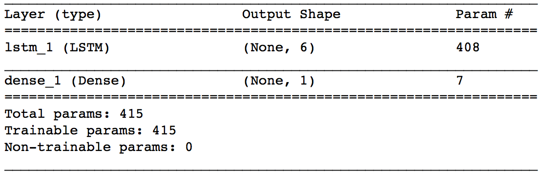
The last layer is a dense layer where the loss is mean squared error with stochastic gradient descent as an optimizer. We train this model for 200 epochs with early_stopping callback. The summary of the model is shown above.

LSTM Prediction

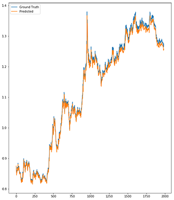
This model has learned to reproduce the yearly shape of the data and doesn’t have the lag it used to have with a simple feed forward neural network. It is still underestimating some observations by certain amounts and there is definitely room for improvement in this model.

Changes in the model

There can be a lot of changes to be made in this model to make it better. One can always try to change the configuration by changing the optimizer. Another important change I see is by using the Sliding Time Window method, which comes from the field of stream data management system.

This approach comes from the idea that only the most recent data are important. One can show the model data from a year and try to make a prediction for the first day of the next year. Sliding time window methods are very useful in terms of fetching important patterns in the dataset that are highly dependent on the past bulk of observations.

Try to make changes to this model as you like and see how the model reacts to those changes.

Dataset

I made the dataset available on my github account under deep learning in python repository. Feel free to download the dataset and play with it.

Useful sources

I personally follow some of my favorite data scientists like Kirill Eremenko, Jose Portilla, Dan Van Boxel (better known as Dan Does Data), and many more. Most of them are available on different podcast stations where they talk about different current subjects like RNN, Convolutional Neural Networks, LSTM, and even the most recent technology, Neural Turing Machine.

Try to keep up with the news of different artificial intelligence conferences. By the way, if you are interested, then Kirill Eremenko is coming to San Diego this November with his amazing team to give talks on Machine Learning, Neural Networks, and Data Science.

Conclusion

LSTM models are powerful enough to learn the most important past behaviors and understand whether or not those past behaviors are important features in making future predictions. There are several applications where LSTMs are highly used. Applications like speech recognition, music composition, handwriting recognition, and even in my current research of human mobility and travel predictions.

According to me, LSTM is like a model which has its own memory and which can behave like an intelligent human in making decisions.

Thank you again and happy machine learning!