92、R语言分析案例
来源:互联网 发布:随机抽取名字软件 编辑:程序博客网 时间:2024/04/29 10:13
1、读取数据
> bank=read.table("bank-full.csv",header=TRUE,sep=";")>
2、查看数据结构
> bank=read.table("bank-full.csv",header=TRUE,sep=",")> str(bank)'data.frame': 41188 obs. of 21 variables: $ age : int 56 57 37 40 56 45 59 41 24 25 ... $ job : Factor w/ 12 levels "admin.","blue-collar",..: 4 8 8 1 8 8 1 2 10 8 ... $ marital : Factor w/ 4 levels "divorced","married",..: 2 2 2 2 2 2 2 2 3 3 ... $ education : Factor w/ 8 levels "basic.4y","basic.6y",..: 1 4 4 2 4 3 6 8 6 4 ... $ default : Factor w/ 3 levels "no","unknown",..: 1 2 1 1 1 2 1 2 1 1 ... $ housing : Factor w/ 3 levels "no","unknown",..: 1 1 3 1 1 1 1 1 3 3 ... $ loan : Factor w/ 3 levels "no","unknown",..: 1 1 1 1 3 1 1 1 1 1 ... $ contact : Factor w/ 2 levels "cellular","telephone": 2 2 2 2 2 2 2 2 2 2 ... $ month : Factor w/ 10 levels "apr","aug","dec",..: 7 7 7 7 7 7 7 7 7 7 ... $ day_of_week : Factor w/ 5 levels "fri","mon","thu",..: 2 2 2 2 2 2 2 2 2 2 ... $ duration : int 261 149 226 151 307 198 139 217 380 50 ... $ campaign : int 1 1 1 1 1 1 1 1 1 1 ... $ pdays : int 999 999 999 999 999 999 999 999 999 999 ... $ previous : int 0 0 0 0 0 0 0 0 0 0 ... $ poutcome : Factor w/ 3 levels "failure","nonexistent",..: 2 2 2 2 2 2 2 2 2 2 ... $ emp.var.rate : num 1.1 1.1 1.1 1.1 1.1 1.1 1.1 1.1 1.1 1.1 ... $ cons.price.idx: num 94 94 94 94 94 ... $ cons.conf.idx : num -36.4 -36.4 -36.4 -36.4 -36.4 -36.4 -36.4 -36.4 -36.4 -36.4 ... $ euribor3m : num 4.86 4.86 4.86 4.86 4.86 ... $ nr.employed : num 5191 5191 5191 5191 5191 ... $ y : Factor w/ 2 levels "no","yes": 1 1 1 1 1 1 1 1 1 1 ...
3、查看摘要统计量
> summary(bank) age job marital education Min. :17.00 admin. :10422 divorced: 4612 university.degree :12168 1st Qu.:32.00 blue-collar: 9254 married :24928 high.school : 9515 Median :38.00 technician : 6743 single :11568 basic.9y : 6045 Mean :40.02 services : 3969 unknown : 80 professional.course: 5243 3rd Qu.:47.00 management : 2924 basic.4y : 4176 Max. :98.00 retired : 1720 basic.6y : 2292 (Other) : 6156 (Other) : 1749 default housing loan contact month no :32588 no :18622 no :33950 cellular :26144 may :13769 unknown: 8597 unknown: 990 unknown: 990 telephone:15044 jul : 7174 yes : 3 yes :21576 yes : 6248 aug : 6178 jun : 5318 nov : 4101 apr : 2632 (Other): 2016 day_of_week duration campaign pdays previous fri:7827 Min. : 0.0 Min. : 1.000 Min. : 0.0 Min. :0.000 mon:8514 1st Qu.: 102.0 1st Qu.: 1.000 1st Qu.:999.0 1st Qu.:0.000 thu:8623 Median : 180.0 Median : 2.000 Median :999.0 Median :0.000 tue:8090 Mean : 258.3 Mean : 2.568 Mean :962.5 Mean :0.173 wed:8134 3rd Qu.: 319.0 3rd Qu.: 3.000 3rd Qu.:999.0 3rd Qu.:0.000 Max. :4918.0 Max. :56.000 Max. :999.0 Max. :7.000 poutcome emp.var.rate cons.price.idx cons.conf.idx failure : 4252 Min. :-3.40000 Min. :92.20 Min. :-50.8 nonexistent:35563 1st Qu.:-1.80000 1st Qu.:93.08 1st Qu.:-42.7 success : 1373 Median : 1.10000 Median :93.75 Median :-41.8 Mean : 0.08189 Mean :93.58 Mean :-40.5 3rd Qu.: 1.40000 3rd Qu.:93.99 3rd Qu.:-36.4 Max. : 1.40000 Max. :94.77 Max. :-26.9 euribor3m nr.employed y Min. :0.634 Min. :4964 no :36548 1st Qu.:1.344 1st Qu.:5099 yes: 4640 Median :4.857 Median :5191 Mean :3.621 Mean :5167 3rd Qu.:4.961 3rd Qu.:5228 Max. :5.045 Max. :5228
> psych::describe(bank) vars n mean sd median trimmed mad min maxage 1 41188 40.02 10.42 38.00 39.30 10.38 17.00 98.00job* 2 41188 4.72 3.59 3.00 4.48 2.97 1.00 12.00marital* 3 41188 2.17 0.61 2.00 2.21 0.00 1.00 4.00education* 4 41188 4.75 2.14 4.00 4.88 2.97 1.00 8.00default* 5 41188 1.21 0.41 1.00 1.14 0.00 1.00 3.00housing* 6 41188 2.07 0.99 3.00 2.09 0.00 1.00 3.00loan* 7 41188 1.33 0.72 1.00 1.16 0.00 1.00 3.00contact* 8 41188 1.37 0.48 1.00 1.33 0.00 1.00 2.00month* 9 41188 5.23 2.32 5.00 5.31 2.97 1.00 10.00day_of_week* 10 41188 3.00 1.40 3.00 3.01 1.48 1.00 5.00duration 11 41188 258.29 259.28 180.00 210.61 139.36 0.00 4918.00campaign 12 41188 2.57 2.77 2.00 1.99 1.48 1.00 56.00pdays 13 41188 962.48 186.91 999.00 999.00 0.00 0.00 999.00previous 14 41188 0.17 0.49 0.00 0.05 0.00 0.00 7.00poutcome* 15 41188 1.93 0.36 2.00 2.00 0.00 1.00 3.00emp.var.rate 16 41188 0.08 1.57 1.10 0.27 0.44 -3.40 1.40cons.price.idx 17 41188 93.58 0.58 93.75 93.58 0.56 92.20 94.77cons.conf.idx 18 41188 -40.50 4.63 -41.80 -40.60 6.52 -50.80 -26.90euribor3m 19 41188 3.62 1.73 4.86 3.81 0.16 0.63 5.04nr.employed 20 41188 5167.04 72.25 5191.00 5178.43 55.00 4963.60 5228.10y* 21 41188 1.11 0.32 1.00 1.02 0.00 1.00 2.00 range skew kurtosis seage 81.00 0.78 0.79 0.05job* 11.00 0.45 -1.39 0.02marital* 3.00 -0.06 -0.34 0.00education* 7.00 -0.24 -1.21 0.01default* 2.00 1.44 0.07 0.00housing* 2.00 -0.14 -1.95 0.00loan* 2.00 1.82 1.38 0.00contact* 1.00 0.56 -1.69 0.00month* 9.00 -0.31 -1.03 0.01day_of_week* 4.00 0.01 -1.27 0.01duration 4918.00 3.26 20.24 1.28campaign 55.00 4.76 36.97 0.01pdays 999.00 -4.92 22.23 0.92previous 7.00 3.83 20.11 0.00poutcome* 2.00 -0.88 3.98 0.00emp.var.rate 4.80 -0.72 -1.06 0.01cons.price.idx 2.57 -0.23 -0.83 0.00cons.conf.idx 23.90 0.30 -0.36 0.02euribor3m 4.41 -0.71 -1.41 0.01nr.employed 264.50 -1.04 0.00 0.36y* 1.00 2.45 4.00 0.00
4、查看数据是否有缺失
> sapply(bank,anyNA) age job marital education default FALSE FALSE FALSE FALSE FALSE housing loan contact month day_of_week FALSE FALSE FALSE FALSE FALSE duration campaign pdays previous poutcome FALSE FALSE FALSE FALSE FALSE emp.var.rate cons.price.idx cons.conf.idx euribor3m nr.employed FALSE FALSE FALSE FALSE FALSE y FALSE >
5、单变量频数分析
> table(bank$y) no yes 36548 4640 >
6、两个变量的交叉列联表
> table(bank$y,bank$marital) divorced married single unknown no 4136 22396 9948 68 yes 476 2532 1620 12>
> xtabs(~y+marital,data=bank) maritaly divorced married single unknown no 4136 22396 9948 68 yes 476 2532 1620 12>
7、
> prop.table(tab,1) divorced married single unknown no 0.113166247 0.612783189 0.272189997 0.001860567 yes 0.102586207 0.545689655 0.349137931 0.002586207> prop.table(tab,2) divorced married single unknown no 0.8967910 0.8984275 0.8599585 0.8500000 yes 0.1032090 0.1015725 0.1400415 0.1500000>
8、构建更复杂的Table
> ftable(bank[,c(3,4,21)],row.vars = c(1,2),col.vars = "y") y no yesmarital education divorced basic.4y 406 83 basic.6y 169 13 basic.9y 534 31 high.school 1086 107 illiterate 1 1 professional.course 596 61 university.degree 1177 160 unknown 167 20married basic.4y 2915 313 basic.6y 1628 139 basic.9y 3858 298 high.school 4683 475 illiterate 12 3 professional.course 2799 357 university.degree 5573 821 unknown 928 126single basic.4y 422 31 basic.6y 301 36 basic.9y 1174 142 high.school 2702 448 illiterate 1 0 professional.course 1247 177 university.degree 3723 683 unknown 378 103unknown basic.4y 5 1 basic.6y 6 0 basic.9y 6 2 high.school 13 1 illiterate 0 0 professional.course 6 0 university.degree 25 6 unknown 7 2>
9、卡方检验
> tab divorced married single unknown no 4136 22396 9948 68 yes 476 2532 1620 12
> chisq.test(tab) Pearson's Chi-squared testdata: tabX-squared = 122.66, df = 3, p-value < 2.2e-16>
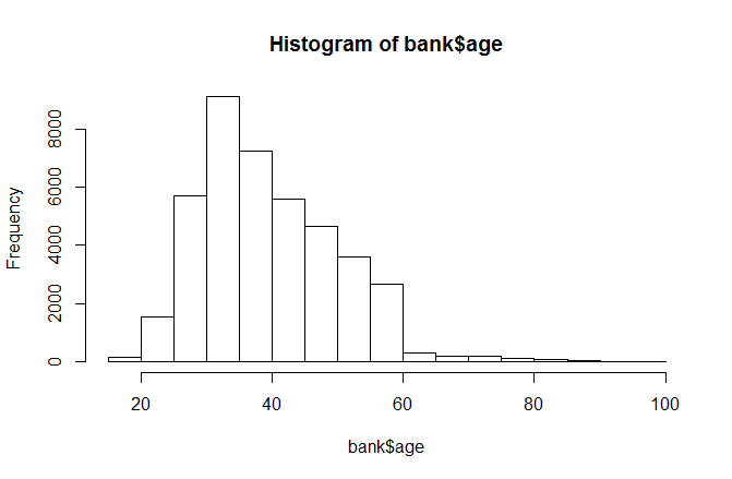
10、连续数据可视化
> hist(bank$age)>
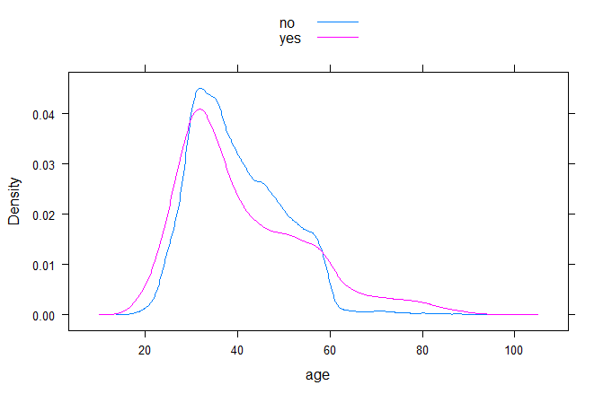
11、连续变量的分布
> library(lattice)> densityplot(~age,groups=y,data=bank,plot.point=FALSE,auto.key = TRUE)>
阅读全文
0 0
- 92、R语言分析案例
- R语言实用案例分析-1
- R语言生存分析数据分析可视化案例
- R语言案例分析:多元数据的基本统计分析
- R语言实用案例分析-相关系数的应用
- R语言案例分析:财政收入的多元相关与回归分析
- R语言快速入门_案例分析之考试成绩的回归分析
- R语言 shiny企业轻量级可视化应用案例(R语言&大数据分析qq群 456726635 欢迎讨论交流)
- R语言多元分析
- R语言-回归分析
- R语言 股价分析
- R语言-文本分析
- R语言相关分析
- R语言生存分析
- R语言回归分析
- R语言关联分析
- R语言-生存分析
- R语言t检验,秩和检验,fdr的案例分析
- poj2457 Part Acquisition
- 89、tensorflow使用GPU并行计算
- 90、Tensorflow实现分布式学习,多台电脑,多个GPU 异步试学习
- 重构的那些事儿
- 91、R语言编程基础
- 92、R语言分析案例
- LED设备驱动开发实验—源码代码详解
- 93、R语言教程详解
- 搭建Spring Boot项目(mybatis、druid、自定义消息转换等)
- 94、tensorflow实现语音识别0,1,2,3,4,5,6,7,8,9
- Jmeter使用SSL(HTTPS协议)
- 95、自然语言处理svd词向量
- leetcode 48
- cs224d 作业 problem set1 (二) 简单的情感分析