Python机器学习房价预测 (斯坦福大学机器学习课程)

问题来自慕课斯坦福机器学习课程
更多机器学习内容访问omegaxyz.com

问题

·输入数据只有一维：房子的面积
·目标的数据只有一维：房子的价格
根据已知房子的面积和价格进行机器学习和模型预测
数据见文章末尾
数据需要标准化X=(X-aver(sum(Xi)))/std(Xi)

步骤①数据获取与处理

# 导入需要用到的库import numpy as npimport matplotlib.pyplot as plt# 定义存储输入数据（x）和目标数据（y）的数组x, y = [], []# 遍历数据集，变量sample对应的正是一个个样本for sample in open("C:\\Users\\dell\\Desktop\\house_prices.txt", 'r'):    _x, _y = sample.split(",")    # 将字符串数据转化为浮点数    x.append(float(_x))    y.append(float(_y))# 读取完数据后，将他们转化为Numpy数组以方便进一步的处理x, y = np.array(x), np.array(y)# 标准化x = (x - x.mean()) / x.std()# 将原始数据集以散点的形式画出plt.figure()plt.scatter(x, y, c="g", s=6)plt.show()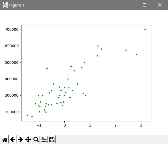

横轴是标准化之后的面积，纵轴是房子的价格

步骤②选择与训练模型

模型损失函数是平方损失函数也就是所谓的欧式距离，这里的目的是要将损失函数最小化
利用Numpy训练和优化

模型的数学表达式为：
f(x|p;n)=p0x^n+p1x^(n-1)+…+pn-1x+pn
L(p;n)=0.5∑[f(x|p;n)-y]^2

# (-2,4)这个区间上取100个点作为画图的基础x0 = np.linspace(-2, 4, 100)# 利用Numpy的函数定义训练并返回多项式回归模型的次数# deg参数代表着模型参数中的n，即模型中多项式的次数# 返回的模型能够根据输入的x（默认是x0）,返回预测的ydef get_model(deg):    return lambda input_x=x0: np.polyval(np.polyfit(x, y ,deg), input_x)

步骤③评估与显示

多项式拟合，采用n=1,4,10进行评估
不需要进行交叉验证因为数据太少了

# 根据参数n、输入的x,y返回相对应的损失def get_cost(deg, input_x,input_y):    return 0.5 * ((get_model(deg)(input_x) - input_y) ** 2).sum()# 定义测试函数集并根据它进行各种实验test_set = (1, 4, 10)for d in test_set:    # 输出损失    print(get_cost(d, x, y))# 画出相应的图像plt.scatter(x, y, c="g", s=20)for d in test_set:    plt.plot(x0, get_model(d)(), label="degree = {}".format(d))# 将横轴和纵轴的范围分别限制在(-2,4)和(10^5,10^6)plt.xlim(-2, 4)plt.ylim(1e5, 1e6)# 调用legend方法使曲线对应的label正确显示plt.legend()plt.show()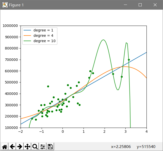

当n=4和10时出现过拟合现象，因此n=1是预测较好的模型

完整代码

# 导入需要用到的库import numpy as npimport matplotlib.pyplot as plt# 定义存储输入数据（x）和目标数据（y）的数组x, y = [], []# 遍历数据集，变量sample对应的正是一个个样本for sample in open("C:\\Users\\dell\\Desktop\\house_prices.txt", 'r'):    _x, _y = sample.split(",")    # 将字符串数据转化为浮点数    x.append(float(_x))    y.append(float(_y))# 读取完数据后，将他们转化为Numpy数组以方便进一步的处理x, y = np.array(x), np.array(y)# 标准化x = (x - x.mean()) / x.std()# 将原始数据集以散点的形式画出plt.figure()plt.scatter(x, y, c="g", s=6)plt.show()# (-2,4)这个区间上取100个点作为画图的基础x0 = np.linspace(-2, 4, 100)# 利用Numpy的函数定义训练并返回多项式回归模型的次数# deg参数代表着模型参数中的n，即模型中多项式的次数# 返回的模型能够根据输入的x（默认是x0）,返回预测的ydef get_model(deg):    return lambda input_x=x0: np.polyval(np.polyfit(x, y ,deg), input_x)# 根据参数n、输入的x,y返回相对应的损失def get_cost(deg, input_x,input_y):    return 0.5 * ((get_model(deg)(input_x) - input_y) ** 2).sum()# 定义测试函数集并根据它进行各种实验test_set = (1, 4, 10)for d in test_set:    # 输出损失    print(get_cost(d, x, y))# 画出相应的图像plt.scatter(x, y, c="g", s=20)for d in test_set:    plt.plot(x0, get_model(d)(), label="degree = {}".format(d))# 将横轴和纵轴的范围分别限制在(-2,4)和(10^5,10^6)plt.xlim(-2, 4)plt.ylim(1e5, 1e6)# 调用legend方法使曲线对应的label正确显示plt.legend()plt.show()

参考文献

Python与机器学习实战 何宇健
更多机器学习内容访问omegaxyz.com

数据集

在桌面创建txt文件，注意代码中的路径

house_prices.txt

2104,399900
1600,329900
2400,369000
1416,232000
3000,539900
1985,299900
1534,314900
1427,198999
1380,212000
1494,242500
1940,239999
2000,347000
1890,329999
4478,699900
1268,259900
2300,449900
1320,299900
1236,199900
2609,499998
3031,599000
1767,252900
1888,255000
1604,242900
1962,259900
3890,573900
1100,249900
1458,464500
2526,469000
2200,475000
2637,299900
1839,349900
1000,169900
2040,314900
3137,579900
1811,285900
1437,249900
1239,229900
2132,345000
4215,549000
2162,287000
1664,368500
2238,329900
2567,314000
1200,299000
852,179900
1852,299900
1203,239500

更多机器学习内容访问omegaxyz.com