All of Recurrent Neural Networks (RNN)

— notes for the Deep Learning book, Chapter 10 Sequence Modeling: Recurrent and Recursive Nets.

Meta info: I’d like to thank the authors of the original book for their great work. For brevity, the figures and text from the original book are used without reference. Also, many thanks to colan and shi for their excellent blog posts on LSTM, from which we use some figures.

Introduction

Recurrent Neural Networks (RNN) are for handling sequential data.

RNNs share parameters across different positions/ index of time/ time steps of the sequence, which makes it possible to generalize well to examples of different sequence length. RNN is usually a better alternative to position-independent classifiers and sequential models that treat each position differently.

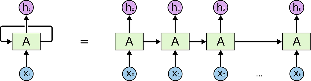
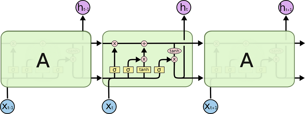
How does a RNN share parameters? Each member of the output is produced using the same update rule applied to the previous outputs. Such update rule is often a (same) NN layer, as the “A” in the figure below (fig from colan).

Notation: We refer to RNNs as operating on a sequence that contains vectors x(t) with the time step index t ranging from 1 to τ. Usually, there is also a hidden state vector h(t) for each time step t.

10.1 Unfolding Computational Graphs

Basic formula of RNN (10.4) is shown below:

It basically says the current hidden state h(t) is a function f of the previous hidden state h(t-1) and the current input x(t). The theta are the parameters of the function f. The network typically learns to use h(t) as a kind of lossy summary of the task-relevant aspects of the past sequence of inputs up to t.

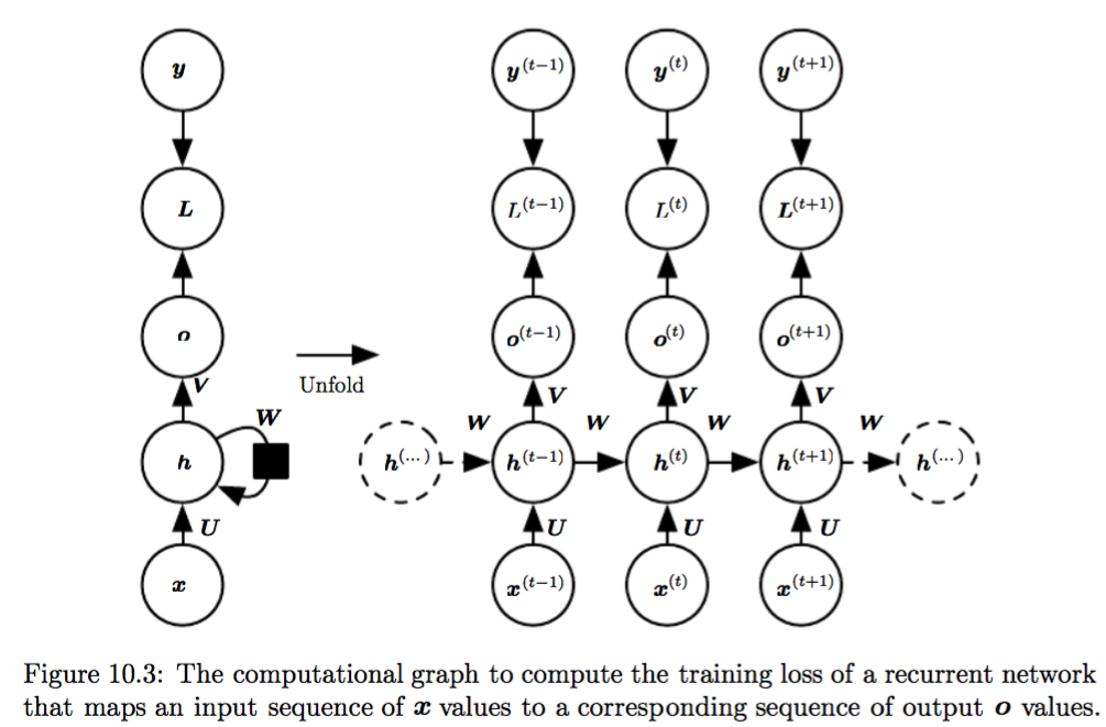
Unfolding maps the left to the right in the figure below (both are computational graphs of a RNN without output o)

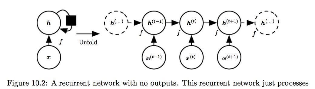
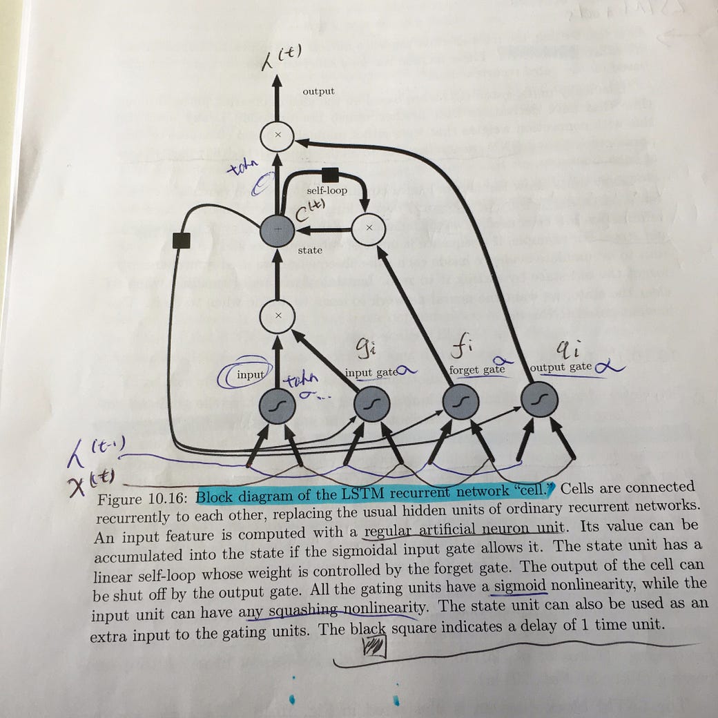
where the black square indicates that an interaction takes place with a delay of 1 time step, from the state at time t to the state at time t + 1.

Unfolding/parameter sharing is better than using different parameters per position: less parameters to estimate, generalize to various length.

10.2 Recurrent Neural Network

Variation 1 of RNN (basic form): hidden2hidden connections, sequence output. As in Fig 10.3.

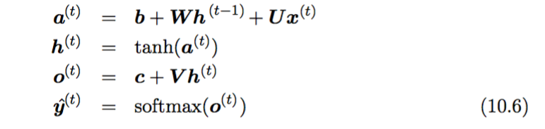
The basic equations that defines the above RNN is shown in (10.6) below (on pp. 385 of the book)

The total loss for a given sequence of x values paired with a sequence of yvalues would then be just the sum of the losses over all the time steps. For example, if L(t) is the negative log-likelihood

of y (t) given x (1), . . . , x (t) , then sum them up you get the loss for the sequence as shown in (10.7):

• Foward Pass: The runtime is O(τ) and cannot be reduced by parallelization because the forward propagation graph is inherently sequential; each time step may only be computed after the previous one.
• Backward Pass: see Section 10.2.2.

Variation 2 of RNN output2hidden, sequence output. As shown in Fig 10.4, it produces an output at each time step and have recurrent connections only from the output at one time step to the hidden units at the next time step

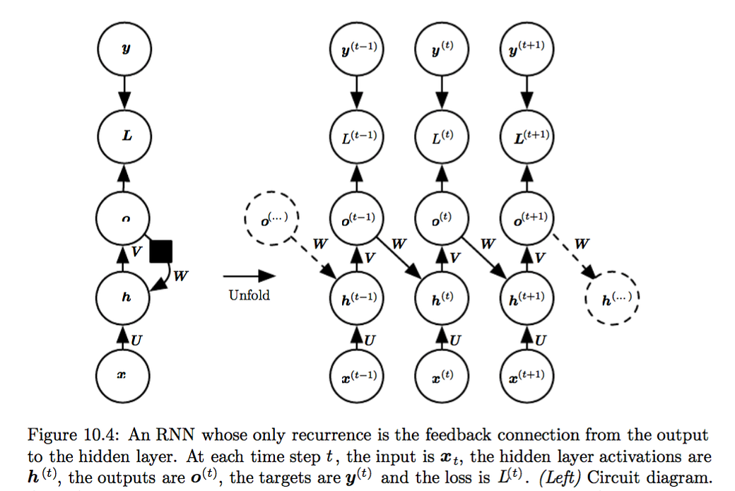
Teacher forcing (Section 10.2.1, pp 385) can be used to train RNN as in Fig 10.4 (above), where only output2hidden connections exist, i.e hidden2hidden connections are absent.

In teach forcing, the model is trained to maximize the conditional probability of current output y(t), given both the x sequence so far and the previous output y(t-1), i.e. use the gold-standard output of previous time step in training.

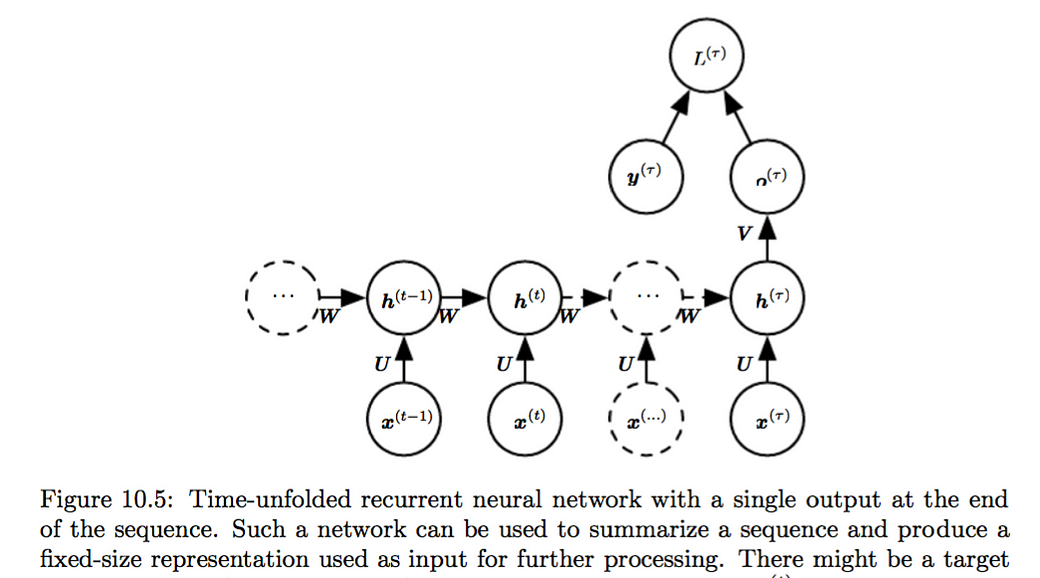
Variation 3 of RNN hidden2hidden, single output. As Fig 10.5 recurrent connections between hidden units, that read an entire sequence and then produce a single output

10.2.2 Computing the Gradient in a Recurrent Neural Network

How? Use back-propagation through time (BPTT) algorithm on on the unrolled graph. Basically, it is the application of chain-rule on the unrolled graph for parameters of U, V , W, b and c as well as the sequence of nodes indexed by t for x(t), h(t), o(t) and L(t).

Hope you find the following derivations elementary….. If not, reading the book probably does NOT help, either

The derivations are w.r.t. the basic form of RNN, namely Fig 10.3 and Equation (10.6) . We copy Fig 10.3 again here:

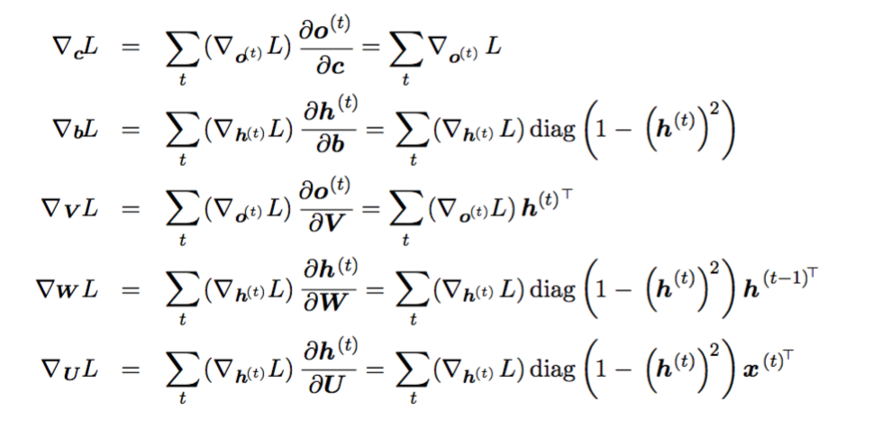
from PP 389:

Once the gradients on the internal nodes of the computational graph are obtained, we can obtain the gradients on the parameter nodes, which have descendents at all the time steps:

PP 390:

Note: We move Section 10.2.3 and Sec 10.2.4, both of which are about graphical model interpretation of RNN, to the end of the notes, as they are not essential for the idea flow, in my opinion…

Note2: One may want to jump to Section 10.7 and read till the end before coming back to 10.3–10.6, as those sections are in parallel with Sections 10.7–10.13, which coherently centers on the long dependency problem.

10.3 Bidirectional RNNs

In many applications we want to output a prediction of y (t) which may depend on the whole input sequence. E.g. co-articulation in speech recognition, right neighbors in POS tagging, etc.

Bidirectional RNNs combine an RNN that moves forward through time beginning from the start of the sequence with another RNN that moves backward through time beginning from the end of the sequence.

Fig. 10.11 (below) illustrates the typical bidirectional RNN, where h(t) and g(t) standing for the (hidden) state of the sub-RNN that moves forward and backward through time, respectively. This allows the output units o(t) to compute a representation that depends on both the past and the future but is most sensitive to the input values around time t

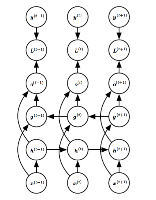
Figure 10.11: Computation of a typical bidirectional recurrent neural network, meant to learn to map input sequences x to target sequences y, with loss L(t) at each step t.

Footnote: This idea can be naturally extended to 2-dimensional input, such as images, by having four RNNs…

10.4 Encoder-Decoder Sequence-to-Sequence Architectures

Encode-Decoder architecture, basic idea:

(1) an encoder or reader or input RNN processes the input sequence. The encoder emits the context C , usually as a simple function of its final hidden state.

(2) a decoder or writer or output RNN is conditioned on that fixed-length vector to generate the output sequence Y = ( y(1) , . . . , y(ny ) ).

highlight: the lengths of input and output sequences can vary from each other. Now widely used in machine translation, question answering etc.

See Fig 10.12 below.

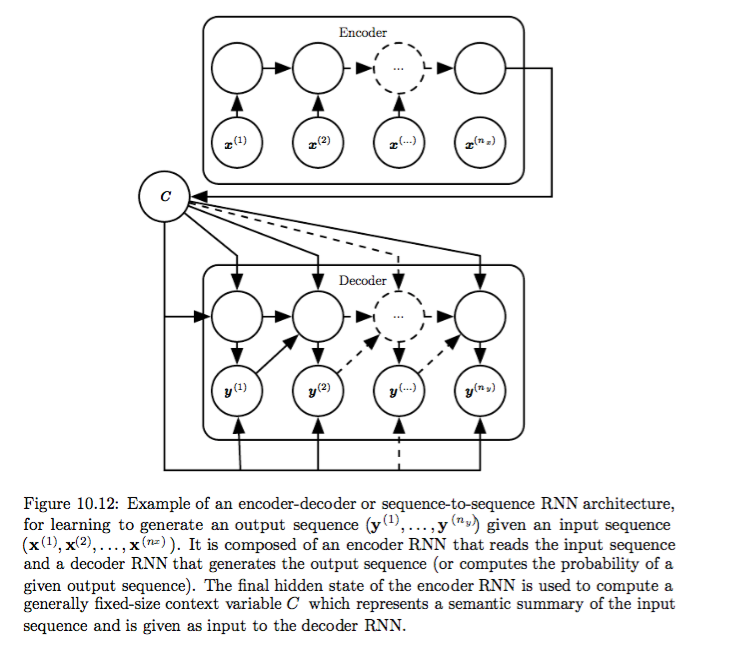
Training: two RNNs are trained jointly to maximize the average of logP(y(1),…,y(ny) |x(1),…,x(nx)) over all the pairs of x and y sequences in the training set.

Variations: If the context C is a vector, then the decoder RNN is simply a vector-to- sequence RNN. As we have seen (in Sec. 10.2.4), there are at least two ways for a vector-to-sequence RNN to receive input. The input can be provided as the initial state of the RNN, or the input can be connected to the hidden units at each time step. These two ways can also be combined.

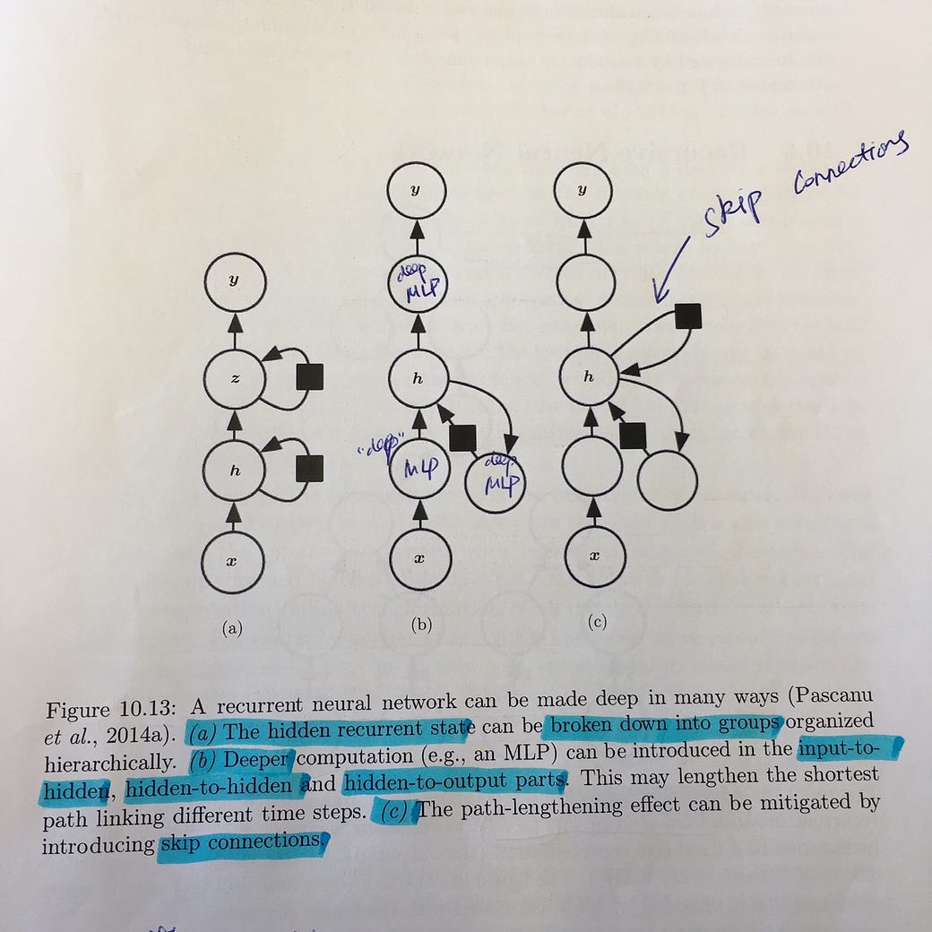
10.5 Deep Recurrent Networks

The computation in most RNNs can be decomposed into three blocks of parameters and associated transformations:

1. from the input to the hidden state, x(t) → h(t)

2. from the previous hidden state to the next hidden state, h(t-1) → h(t)

3. from the hidden state to the output, h(t) → o(t)

These transformations are represented as a single layer within a deep MLP in the previous discussed models. However, we can use multiple layers for each of the above transformations, which results in deep recurrent networks.

Fig 10.13 (below) shows the resulting deep RNN, if we

(a) break down hidden to hidden,

(b) introduce deeper architecture for all the 1,2,3 transformations above and

(c) add “skip connections” for RNN that have deep hidden2hidden transformations.

10.6 Recursive Neural Network

A recursive network has a computational graph that generalizes that of the recurrent network from a chain to a tree.

Pro: Compared with a RNN, for a sequence of the same length τ, the depth (measured as the number of compositions of nonlinear operations) can be drastically reduced from τ to O(logτ).

Con: how to best structure the tree? Balanced binary tree is an optional but not optimal for many data. For natural sentences, one can use a parser to yield the tree structure, but this is both expensive and inaccurate. Thus recursive NN is NOT popular.

10.7 The challenge of Long-Term Dependency

• Comments: This is the central challenge of RNN, which drives the rest of the chapter.

The long-term dependency challenge motivates various solutions such as Echo state network (Section 10.8), leaky units (Sec 10.9) and the infamous LSTM(Sec 10.10), as well as clipping gradient, neural turing machine (Sec 10.11).

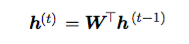
Recurrent networks involve the composition of the same function multiple times, once per time step. These compositions can result in extremely nonlinear behavior. But let’s focus on a linear simplification of RNN, where all the non-linearity are removed, for an easier demonstration of why long-term dependency can be problematic.

Without non-linearity, the recurrent relation for h(t) w.r.t. h(t-1) is now simply matrix multiplication:

If we recurrently apply this until we reach h(0), we get:

and if W admits an eigen-decomposition

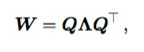
the recurrence may be simplified further to:

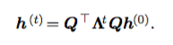
In other words, the recurrence means that the eigenvalues are raised to the power of t. This means that eigenvalues with magnitude less than one to vanish to zero and eigenvalues with magnitude greater than one to explode. The above analysis shows the essence of the vanishing and exploding gradient problem for RNNs.

Comment: the trend of recurrence in matrix multiplication is similar in actual RNN, if we look back at 10.2.2 “Computing the Gradient in a Recurrent Neural Network”.

Bengio et al., (1993, 1994) shows that whenever the model is able to represent long term dependencies, the gradient of a long term interaction has exponentially smaller magnitude than the gradient of a short term interaction. It means that it can be time-consuming, if not impossible, to learn long-term dependencies. The following sections are all devoted to solving this problem.

Practical tips: The maximum sequences length that SGD-trained traditional RNN can handle is only 10 ~ 20.

10.8 Echo State Networks

Note: This approach seems to be non-salient in the literature, so knowing the concept is probably enough. The techniques are only explained at an abstract level in the book, anyway.

Basic Idea: Since the recurrence causes all the vanishing/exploding problems, we can set the recurrent weights such that the recurrent hidden units do a good job of capturing the history of past inputs (thus “echo”), and only learn the output weights.

Specifics: The original idea was to make the eigenvalues of the Jacobian of the state-to-

state transition function be close to 1. But that is under the assumption of no non-linearity. So The modern strategy is simply to fix the weights to have some spectral radius such as 3, where information is carried forward through time but does not explode due to the stabilizing effect of saturating nonlinearities like tanh.

10.9 Leaky Units and Other Strategies for Multiple Time Scales

A common idea shared by various methods in the following sections: design a model that operates on both fine time scale (handle small details) and coarse time scale (transfer information through long-time).

• Adding skip connections. One way to obtain coarse time scales is to add direct connections from variables in the distant past to variables in the present. Not an ideal solution.

10.9.2 Leaky Units

Idea: each hidden state u(t) is now a “summary of history”, which is set to memorize both a coarse-grained immediate past summary of history u(t-1)and some “new stuff” of present time v(t):

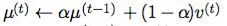
where alpha is a parameter. Then this introduces a linear self-connections from u(t-1) → u(t), with a weight of alpha.

In this case, the alpha substitutes the matrix W’ of the plain RNN (in the analysis of Sec 10.7 ). So if alpha ends up near 1, the several multiplications will not leads to zero or exploded number.

Note: The notation seems to suggest alpha is a scalar, but it looks it will also work if alpha is a vector and the multiplications there is element-wise, which will resemble gate recurrent unit (GRU) as in the coming Section 10.10.

• Removing Connections: actively removing length-one connections and replacing them with longer connections

10.10 The Long Short-Term Memory and Other Gated RNNs

The most effective sequence models used in practice are called gated RNNs. These include the long short-term memory (LSTM) and networks based on the gated recurrent unit (GRU).

Key insight of gated RNN: Gated RNNs allow the neural network to forgetthe old state, besides accumulating info (as leaky units can also do).

10.10.1 LSTM

Long short-term memory (LSTM) model (Hochreiter and Schmidhuber, 1997) weight the self-loop in RNN conditioned on the context, rather than a fixed way of self-looping.

Recap of plain/vanilla RNN: The current hidden state h(t) of the vanilla RNN is generated from the previous hidden state h(t-1) and the current input x(t)by the basic equation of RNN (10.6), repeated as follows:

• a(t) = b+ Wh(t-1)+Ux(t)
• h(t) = tahn ( a(t) )

Due to the properties of block matrix, this is equivalent to feeding the concatenation of [h(t-1), x(t), b] to a single linear (dense) layer being parameterized by a single matrix, which has a tahn non-linearity.

What’s new in LSTM

By contrast, the LSTM uses a group of layers to generate the current hidden state h(t). In short, the extra elements in LSTM include:

• an extra state C(t) is introduced to keep track of the current “history”.
• this C(t) is the sum of the weighted previous history C(t-1) and the weighted “new stuff”, the latter of which is generated similarly as the h(t)in a plain RNN.
• the weighted C(t) yields the current hidden state h(t).

As mentioned earlier, such weighting is conditioned on the context. In LSTM, this is done by the following gates, those information (signal) flow out from yellow-colored sigmoid nodes in the following figure (Fig: LSTM), from left to right:

1. the forget gate f that controls how much previous “history” C(t-1) flows into the current “history”.
2. the external input gate g that controls how much “new stuff” flows into the new “history”
3. the output gate q that controls how much current “history” C(t) follows into the current hidden states h(t)

The actual control by the gate signal occurs at the blue-colored element-wise multiplication nodes, where the control signal from gates are element-wisely multiplied with the states to be weighted: the “previous history” C(t-1), the“new stuff” (output of the left tahn node) and the “current history” C(t)after the right tahn non-linearity , respectively, in a left-to-right order.

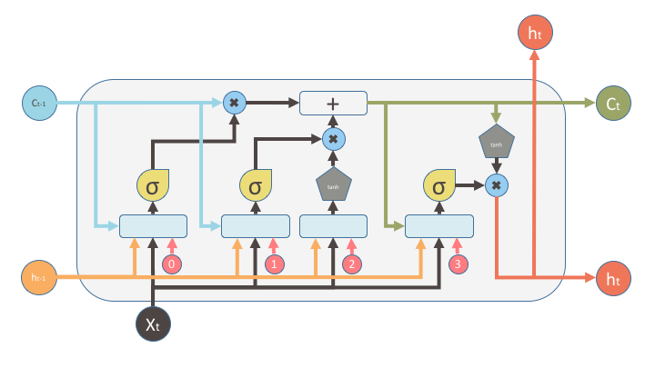
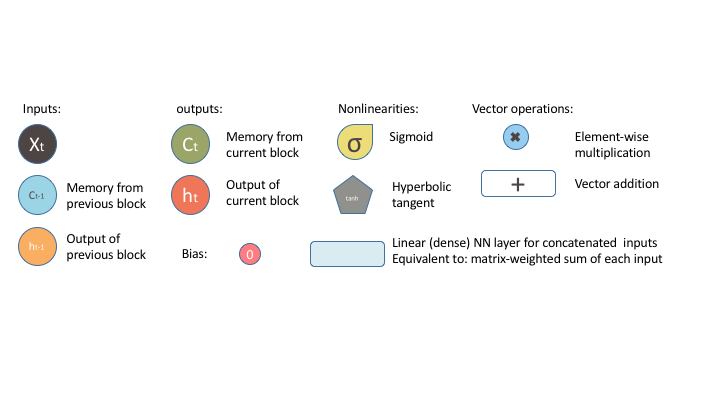
Fig: LSTM, adapted from shi.

• Why the self-loop in LSTM is said to be conditioned the context? This context here simply consists of the current input x(t) and the previous hidden state h(t-1). All the gates use the same input context, namely the concatenation of [h(t-1), x(t)], although each gate has its own bias vector.

Here is another illustration of LSTM from colah, as follows, which is equivalent as the above illustration, although more compact (thus slightly more difficult to read):

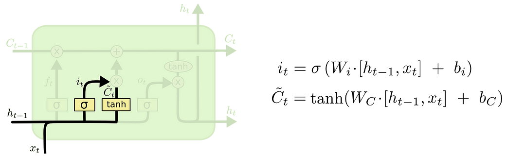
What’s nice about the Colah figure and his blog post itself is that it shows how to break down LSTMs and how to related the figure with the equations. Here’s my summary of the break-down (fig from Colah):

1. The forget gate f(t). The formula maps to (10.25) in the book. Again, note the equivalence caused by block matrix properties (this applies to for all equations from the Colah post). In our case, this Wf below can be blocked into [U, W], which are the notations/matrix used in the the book.

1. The “new stuff”, tilda C(t) in the formula below, is weighted by the external input gate i(t). This maps to formula (10.27) and the rightmost term in (10.26) of the book, where the external input gate is denoted as g(t).

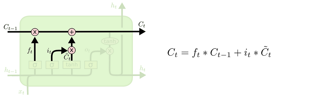
1. How the previous “history”, C(t-1) and “new stuff”, tilda C(t) are weighted by the forget gate f and external input gate i (which is denoted as g(t) in the book), respectively, before they are added together to form form the current “history” C(t).

4. Finally, how the current “history” C(t) goes through a tahn non-linearity and is then weighted by the output gate o(t) (which is denoted as q(t) in the book).

Note: the formula (10.25) — (10.28) in the book are written in a component-wise, non-vectorized form, thus the underscript i in each term.

Hopefully, how LSTM works is clear by now. If not, I recommend to read the colah blog post. And finally, here’s my annotation of the Fig 10.16 in the book, which might make better sense now.

10.10.2 Other Gated RNN

If you find LSTM too complicated, gated recurrent units or GRUs might be your cup of tea. The update rule of GRU can be described in a one-linear (10.29):

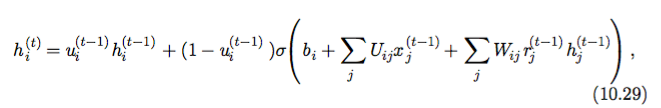
• Obviously, u(t) is a gate (called update gate) here, which decides how much the previous hidden state h(t-1) goes into the current one h(t) and at the same time how much the “new stuff” (the rightmost term in the formula) goes into the current hidden state.
• There is yet another gate r(t), called reset gate, which decides how much the previous state h(t-1) goes into the “new stuff”.

Note: If reset gate were absent, GRU would look very similar to the leaky units, although (1) u(t) is a vector that can weight each dim separately, while alpha in the leaky unit is likely to be a scalar and (2) u(t) is context-dependent, a function of h(t-1) and x(t).

• This ability to forget via the reset gate is found to be essential, which is also true for the forget gate of LSTM.

Practical tips: LSTM is still the best-performing RNN so far. GRU preforms slightly worse than LSTM but better than plain RNN in many applications. It is often a good practice to set the bias of the forget gate of LSTM to 1 (another saying is 0.5 will do for initialization ).

10.11 Optimization for Long-Term Dependencies

Notes: these techniques here are not quite useful nowadays, since most of the time using LSTM will solve the long-term dependency problem. Nevertheless, it is good to know the old tricks.

Take-away: It is often much easier to design a model that is easy to optimizethan it is to design a more powerful optimization algorithm.

Clipping gradient avoids gradient explode but NOT gradient vanish. One option is to clip the parameter gradient from a minibatch element-wise (Mikolov, 2012) just before the parameter update. Another is to clip the norm ||g|| of the gradient g (Pascanu et al., 2013a) just before the parameter update.

Regularizing to encourage the information flow. Favor gradient vector being back-propagated to maintain its magnitude, i.e. penalize the L2 norm differences between such vectors.

10.13 Explicit Memory

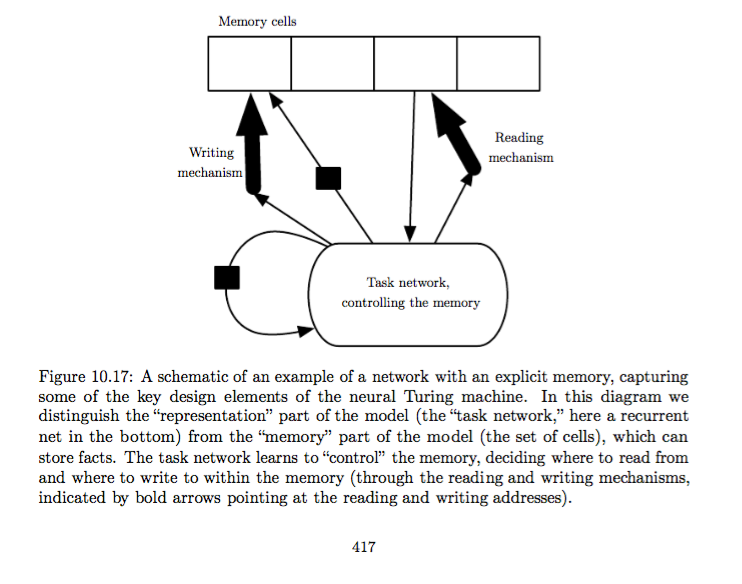
Neural networks excel at storing implicit knowledge. However, they struggle to memorize facts. So it is often helpful to introduce explicit memory component, not only to rapidly and “intentionally” store and retrieve specific facts but also to sequentially reason with them.

• Memory networks (Weston et al. 2014) include a set of memory cells that can be accessed via an addressing mechanism, which requires a supervision signal instructing them how to use their memory cells.
• Neural Turing machine (Graves et al. (2014b)), which is able to learn to read from and write arbitrary content to memory cells without explicit supervision about which actions to undertake.

Neural Turing machine (NTM) allows end-to-end training without external supervision signal, thanks the use of a content-based soft attention mechanism (Bahdanau et al., 2014)). It is difficult to optimize functions that produce exact, integer addresses. To alleviate this problem, NTMs actually read to or write from many memory cells simultaneously.

Note: It might make better sense to read the original paper to understand NTM. Nevertheless, here’s a illustrative graph:

============ Now we visit 10.2.3 and 10.2.4 in detail

10.2.3 Recurrent Networks as Directed Graphical Models

This section is only useful for understanding RNN from a probabilistic graphic model perspective. Can be ignored… We can jump this section and the next (10.2.4) pp390- pp398

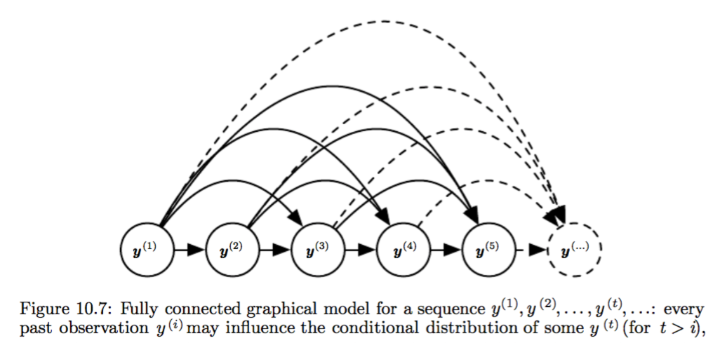
The point of this section seems to show that RNN provides a very efficient parametrization of the joint distribution over the observations.

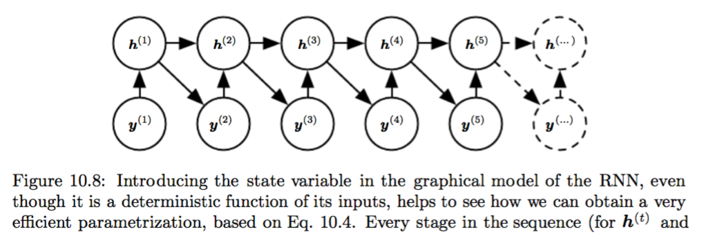
E.g. the introduction of hidden state and hidden2hidden connections can be motivated as reduce Fig 10.7 to Fig 10.8, the latter of which has O(1)*τ parameters while the former has O(k^τ ) parameters. τ is the sequence length here. I feel that such imaginary reduction might be kind of factor graph technique.

Incorporating the h(t) nodes in the graphical model decouples the past and the future, acting as an intermediate quantity between them. A variable y(i) in the distant past may influence a variable y(t) via its effect on h.

10.2.4 Modeling Sequences Conditioned on Context with RNNs

Continuation of the graphical model view of RNN. Can be skipped first and revisit later…

This section extends the graphical model view to represent not only a joint distribution over the y variables but also a conditional distribution over y given x.

How to take only a single vector x as input? When x is a fixed-size vector, we can simply make it an extra input of the RNN that generates the y sequence. Some common ways of providing an extra input to an RNN are:

1. as an extra input at each time step, or
2. as the initial state h (0), or
3. both.

That’s the end of the notes.

原文地址：https://medium.com/@jianqiangma/all-about-recurrent-neural-networks-9e5ae2936f6e